.ipynb .pdf

repository open issue

Binder Colab Live Code

Contents

Working with DataFrames

Now we will go to a territory which might be somewhat familiar if you have previously used R (or Matlab). We will import some packages, read the contents of a file and store it in a data-frame.

Importing packages

One of the great things about python that very often you don ‘t have to implement something yourself. It may be already implemented in the many freely accessible python packages, often referred to as the python ecosystem.

If you are working on your local computer, you can install python packages e.g. with the tools pip or conda.

Inside a notebook, hosted on the cloud (e.g. Google Colab), you can install packages via the following code.

!pip install pandas nilearn

Requirement already satisfied: pandas in /home/tspisak/src/RPN-signature/venv/lib/python3.8/site-packages (1.3.2)
Requirement already satisfied: nilearn in /home/tspisak/src/RPN-signature/venv/lib/python3.8/site-packages (0.8.0)
Requirement already satisfied: python-dateutil>=2.7.3 in /home/tspisak/src/RPN-signature/venv/lib/python3.8/site-packages (from pandas) (2.8.2)
Requirement already satisfied: pytz>=2017.3 in /home/tspisak/src/RPN-signature/venv/lib/python3.8/site-packages (from pandas) (2021.1)
Requirement already satisfied: numpy>=1.17.3 in /home/tspisak/src/RPN-signature/venv/lib/python3.8/site-packages (from pandas) (1.19.5)
Requirement already satisfied: joblib>=0.12 in /home/tspisak/src/RPN-signature/venv/lib/python3.8/site-packages (from nilearn) (1.0.1)
Requirement already satisfied: scipy>=1.2 in /home/tspisak/src/RPN-signature/venv/lib/python3.8/site-packages (from nilearn) (1.7.1)
Requirement already satisfied: requests>=2 in /home/tspisak/src/RPN-signature/venv/lib/python3.8/site-packages (from nilearn) (2.26.0)
Requirement already satisfied: nibabel>=2.5 in /home/tspisak/src/RPN-signature/venv/lib/python3.8/site-packages (from nilearn) (3.2.1)
Requirement already satisfied: scikit-learn>=0.21 in /home/tspisak/src/RPN-signature/venv/lib/python3.8/site-packages (from nilearn) (0.24.2)
Requirement already satisfied: packaging>=14.3 in /home/tspisak/src/RPN-signature/venv/lib/python3.8/site-packages (from nibabel>=2.5->nilearn) (21.0)
Requirement already satisfied: pyparsing>=2.0.2 in /home/tspisak/src/RPN-signature/venv/lib/python3.8/site-packages (from packaging>=14.3->nibabel>=2.5->nilearn) (2.4.7)
Requirement already satisfied: six>=1.5 in /home/tspisak/src/RPN-signature/venv/lib/python3.8/site-packages (from python-dateutil>=2.7.3->pandas) (1.16.0)
Requirement already satisfied: certifi>=2017.4.17 in /home/tspisak/src/RPN-signature/venv/lib/python3.8/site-packages (from requests>=2->nilearn) (2021.5.30)
Requirement already satisfied: charset-normalizer~=2.0.0 in /home/tspisak/src/RPN-signature/venv/lib/python3.8/site-packages (from requests>=2->nilearn) (2.0.4)
Requirement already satisfied: idna<4,>=2.5 in /home/tspisak/src/RPN-signature/venv/lib/python3.8/site-packages (from requests>=2->nilearn) (3.2)
Requirement already satisfied: urllib3<1.27,>=1.21.1 in /home/tspisak/src/RPN-signature/venv/lib/python3.8/site-packages (from requests>=2->nilearn) (1.26.6)
Requirement already satisfied: threadpoolctl>=2.0.0 in /home/tspisak/src/RPN-signature/venv/lib/python3.8/site-packages (from scikit-learn>=0.21->nilearn) (2.2.0)
WARNING: You are using pip version 21.2.4; however, version 22.0.3 is available.
You should consider upgrading via the '/home/tspisak/src/RPN-signature/venv/bin/python -m pip install --upgrade pip' command.

Dependencies in Binder

When launching this notebook interactively via Binder, all dependnecies will already be installed, so this command will have no actual effect. On Google Coleb, there are no costum packages installed, so the rest of this notebook will not function without running this command.

This command installed two packages needed for the rest of this notebook: pandas and nilearn.

Once a package is installed on the system, the only thing we must do is to import the packages, in order to tell python that we intend to use it in your code.

Now, we will import the package called pandas, a package that provides powerful R-like dataframes to store and manipulate your data. For convenience, we also specify that from now on, we would like to refer to pandas as pd, for short.

import pandas as pd

Loading some data

Now let’s load some example data. Throughout the book, we will use brain cortical volume data obtained from the publicly available “Information eXtraction from Images” (IXI) dataset

License info

The IXI dataset is made available under the Creative Commons CC BY-SA 3.0 license. If you use the IXI data please acknowledge the source of the IXI data.

See also

See supplement X for how raw IXI anatomical MRI data was processed with Freesurfer. For more information on analyzing anatomical MR images with Freesurfer e.g. on Andy’s blog.

df=pd.read_csv("https://raw.githubusercontent.com/pni-lab/predmod_lecture/master/ex_data/IXI/ixi.csv")
df

	ID	Age	lh_bankssts_volume	lh_caudalanteriorcingulate_volume	lh_caudalmiddlefrontal_volume	lh_cuneus_volume	lh_entorhinal_volume	lh_fusiform_volume	lh_inferiorparietal_volume	lh_inferiortemporal_volume	...	rh_rostralanteriorcingulate_volume	rh_rostralmiddlefrontal_volume	rh_superiorfrontal_volume	rh_superiorparietal_volume	rh_superiortemporal_volume	rh_supramarginal_volume	rh_frontalpole_volume	rh_temporalpole_volume	rh_transversetemporal_volume	rh_insula_volume
0	2	35.800137	2188	2368	6562	2459	1561	9281	14136	10797	...	2555	17309	21210	12291	12287	10848	1033	2269	1170	6915
1	12	38.781656	2717	2626	6621	3170	2835	8870	14813	11961	...	3260	19044	24651	13871	13948	11975	1100	2865	1167	6941
2	13	46.710472	2101	2488	5437	2347	1859	9200	16900	11675	...	2682	17653	23804	10977	12931	15127	975	2099	1032	7395
3	14	34.236824	1925	1983	5153	2497	2207	7686	12786	8433	...	2120	15070	21001	10993	10890	10453	891	2122	958	6063
4	15	24.284736	2535	1802	5461	2496	1875	6859	14187	7897	...	2825	13027	21865	10651	12686	11400	1185	2207	1344	8218
...	...	...	...	...	...	...	...	...	...	...	...	...	...	...	...	...	...	...	...	...	...
633	648	47.723477	2009	2270	5439	2684	1729	9029	13407	10971	...	3236	15464	21427	11524	12869	11373	814	2419	1360	7423
634	651	50.395619	1776	1532	5797	2954	1992	9131	13201	9005	...	2146	11883	18137	13668	10833	8420	751	2304	1010	6032
635	652	42.989733	2315	1898	6234	3285	1857	10453	15412	10639	...	2931	16905	25113	13148	14489	13440	731	2725	1525	7481
636	653	46.220397	2411	2033	5808	4012	2854	9723	16169	12070	...	2637	15636	19449	13207	13480	11459	1049	2855	1078	7186
637	662	41.741273	2482	1923	4686	3738	1910	10996	16778	10390	...	3492	16781	20968	13379	15787	12850	1069	2521	1062	7931

638 rows × 70 columns

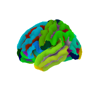
The first two columns of our example dataframe are participant ID and age, then we have a total of 68 cortical volume values, each computed in 34 regions. Rows correspond to participants: a total of N=638. The brain regions were delineated by the as based on the Destrieux brain atlas [5], shown below.

from nilearn import datasets, plotting

destrieux_atlas = datasets.fetch_atlas_surf_destrieux(verbose=0)
fsaverage = datasets.fetch_surf_fsaverage()
plotting.plot_surf_roi(fsaverage['pial_left'], roi_map=destrieux_atlas['map_left'],
                       hemi='left', view='lateral',
                       bg_map=fsaverage['sulc_left'], bg_on_data=True)
plotting.show()

/home/tspisak/src/RPN-signature/venv/lib/python3.8/site-packages/nilearn/datasets/__init__.py:86: FutureWarning: Fetchers from the nilearn.datasets module will be updated in version 0.9 to return python strings instead of bytes and Pandas dataframes instead of Numpy arrays.
  warn("Fetchers from the nilearn.datasets module will be "

Tip

Click on “Click to show” to reveal the python code used for visualizing the atlas. Visualization was done with the python package ‘nilearn’.

See also

Nilearn is a very powerful package for machin elearning with neuroimaging. Check out the nilearn example gallery to have a better impression.

Dataframe slicing

You can get one or multiple columns from a dataframe by slicing it. Let’s extract the age of the participants.

Tip

The output of these commands are hidden by default, click to reveal.

df['Age']

0      35.800137
1      38.781656
2      46.710472
3      34.236824
4      24.284736
         ...    
633    47.723477
634    50.395619
635    42.989733
636    46.220397
637    41.741273
Name: Age, Length: 638, dtype: float64

Now let’s slice the data frame to obtain ID, Age and the volume of the brain region called right superior frontal cortex and obtain the first 5 participants only. To do so you must slice with a list of column names, that’s whz we have double square brackets (outer: slicing, inner: list). Then we call head, to get the ‘head’ of the table.

df_superiorfrontal = df[['ID', 'Age', 'rh_superiorfrontal_volume']]
df_superiorfrontal.head(5)

	ID	Age	rh_superiorfrontal_volume
0	2	35.800137	21210
1	12	38.781656	24651
2	13	46.710472	23804
3	14	34.236824	21001
4	15	24.284736	21865

It is very easy to filter you data frame by the values of one of the columns.

df_superiorfrontal[df_superiorfrontal['Age']>30]

	ID	Age	rh_superiorfrontal_volume
0	2	35.800137	21210
1	12	38.781656	24651
2	13	46.710472	23804
3	14	34.236824	21001
5	16	55.167693	20534
...	...	...	...
633	648	47.723477	21427
634	651	50.395619	18137
635	652	42.989733	25113
636	653	46.220397	19449
637	662	41.741273	20968

534 rows × 3 columns

Plotting

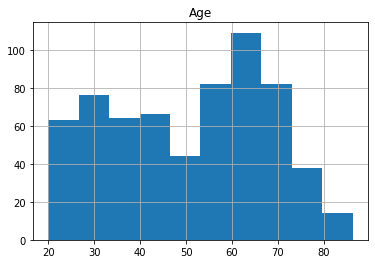
Pandas dataframes provide build-in plotting functions. Let’s see how the age of the participants is distributed.

df.hist('Age')

array([[<AxesSubplot:title={'center':'Age'}>]], dtype=object)

Now, let’s plot the volume of our previously selected brain region against age.

df.plot.scatter(x='Age', y='rh_superiorfrontal_volume')

<AxesSubplot:xlabel='Age', ylabel='rh_superiorfrontal_volume'>

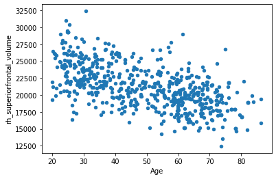
Looks like an inverse association… In the next section, we will see how we can take advantage of this single association in order to predict the age of a participant. And also how we can get into trouble when we want to improve the prediction by adding more regions.

See also

Pandas has an excellent leighweight “Getting Started” tutorial.

Excercise 1.2

Launch this notebook interactively in Google Colab (by clicking the rocket) and modify the code to plot out other variables, e.g. rh_superiorfrontal_volume vs. lh_superiorfrontal_volume.

Excercise 1.3

Launch this notebook interactively in Google Colab (by clicking the rocket) and modify it to load in your own dataset. You can directly upload your dataset file in colab (Select “Files” on the left) or you can also mount your google drive account.

Is you dataframe as Excel spreadsheet? No problem! Check out the function read_excel in pandas.

previous

Introduction to python

next

2. Linear Models and Overfitting