The quickbrain provides fast, lightweight whole-brain surface plotting with a single function call. Unlike most neuroimaging visualisation packages, the built-in MNI152 meshes include the cerebellum and brainstem, giving you a complete overview of brain-wide statistical maps.
Installation
pip install "quickbrain @ git+https://github.com/pni-lab/quickbrain.git"Import
Let’s import the main function plot_brain from the quickbrain package.
from quickbrain import plot_brain1. Quickstart
With no arguments, plot_brain() renders the left pial surface with a
signed-curvature background — gyri and sulci are immediately visible.
The mesh covers the full hemisphere including the cerebellum.
plot_brain()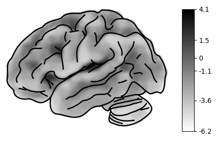
Now we load a statistical map to plot in our examples (in this case meta-analysis of pain responses from Zunhammer et al., 2021).
You can of course use your own data too:
import nibabel as nib
statmap = nib.load("path/to/your/image.nii.gz")
from quickbrain import load_example_image
statmap = load_example_image("pain_response")Pass this to the plot_brain function to plot it.
plot_brain(statmap)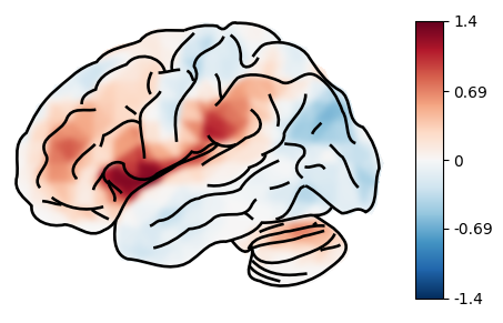
By default, the lateral view of the pial surface of the left hemisphere is plotted. We can change this by passing the following parameters:
hemi:"left"or"right"hemisphere (default:"left")view:"lateral"or"medial"view (default:"lateral")surf_type:"pial"or"inflated"surface type (default:"pial")threshold: the threshold to apply to the statistical map (default:0.0)cmap: the colormap to use (default:"coolwarm")colorbar: whether to show the colorbar (default:True)
Let’s plot the right hemisphere in the medial view with an inflated surface, thresholded at 0.4.
plot_brain(statmap, threshold=0.4, surf_type='inflated', hemi='right', view='medial')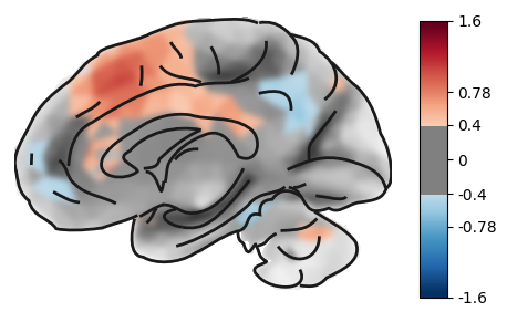
2. Composite plots
quickbrain is fast. So you can plot large composite images, without having to wait a lot for the rendering.
To do so, you can use matplotlib’s subplots to create a grid of plots, and then pass each plot to plot_brain.
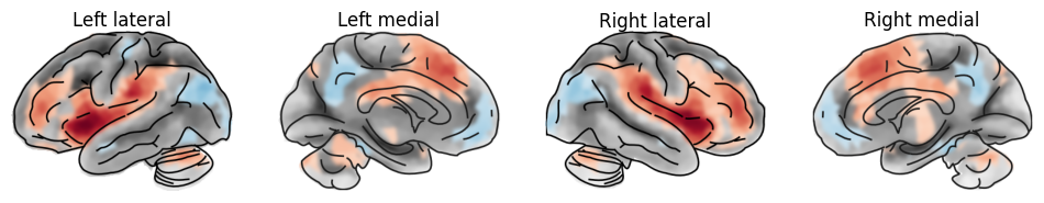
Ideal for visualization during analyses, but also useful for creating overview plots for publications.
import matplotlib.pyplot as plt

_threshold = 0.3
fig, ax = plt.subplots(1, 4, figsize=(12,10), subplot_kw={"projection": "3d"})
plot_brain(statmap, hemi='left', view='lateral', threshold=_threshold, axes=ax[0], colorbar=False, title="Left lateral")
plot_brain(statmap, hemi='left', view='medial', threshold=_threshold, axes=ax[1], colorbar=False, title="Left medial" )
plot_brain(statmap, hemi='right', view='lateral', threshold=_threshold, axes=ax[2], colorbar=False, title="Right lateral")
plot_brain(statmap, hemi='right', view='medial', threshold=_threshold, axes=ax[3], colorbar=False, title="Right medial")
plt.show() 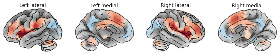
This type of visualization can be useful to show whole brain patterns, e.g. effect sizes, without any thresholding.
_threshold = 0
fig, ax = plt.subplots(1, 4, figsize=(12,10), subplot_kw={"projection": "3d"})
plot_brain(statmap, hemi='left', view='lateral', threshold=_threshold, axes=ax[0], colorbar=False)
plot_brain(statmap, hemi='left', view='medial', threshold=_threshold, axes=ax[1], colorbar=False)
plot_brain(statmap, hemi='right', view='lateral', threshold=_threshold, axes=ax[2], colorbar=False)
plot_brain(statmap, hemi='right', view='medial', threshold=_threshold, axes=ax[3], colorbar=False)
plt.show() 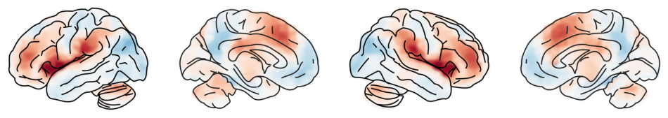
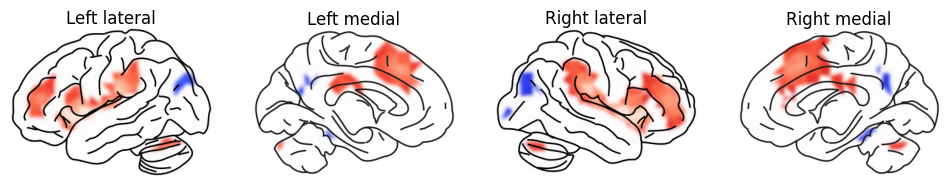
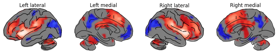
Let’s apply a different style: with a blue-red colormap, thresholded at 0.5, but without the grayscale curvature map, to preserve the clean look, but draw attention to the super-threshold blobs.
import matplotlib.pyplot as plt

_threshold = 0.5
fig, ax = plt.subplots(1, 4, figsize=(12,10), subplot_kw={"projection": "3d"})
plot_brain(statmap, hemi='left', view='lateral', threshold=_threshold, axes=ax[0], cmap='blue_red', colorbar=False, bg_map=0.01, title="Left lateral")
plot_brain(statmap, hemi='left', view='medial', threshold=_threshold, axes=ax[1], cmap='blue_red', colorbar=False,  bg_map=0.01, title="Left medial" )
plot_brain(statmap, hemi='right', view='lateral', threshold=_threshold, axes=ax[2], cmap='blue_red', colorbar=False, bg_map=0.01, title="Right lateral")
plot_brain(statmap, hemi='right', view='medial', threshold=_threshold, axes=ax[3], cmap='blue_red', colorbar=False, bg_map=0.01, title="Right medial")
plt.tight_layout()
plt.show()
/var/folders/rc/b4064_3d4dj60wt9y_447fyr0000gn/T/ipykernel_55088/494689093.py:9: UserWarning: This figure includes Axes that are not compatible with tight_layout, so results might be incorrect.
plt.tight_layout()
On the medial view, we can also see the hippocampus and - with the correct sampling parameters (see later) - signal fromall the subcortical structures.
hip = load_example_image("left_hippocampus")

plot_brain(hip, view='medial', threshold=30, cmap='viridis')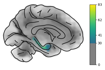
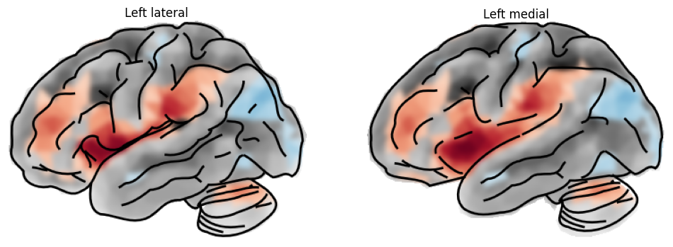
3. Inflated surfaces
With the surf_type parameter, we can switch between the pial and inflated surfaces. The inflated surface provides a better view of deep sulcal structure, for instance the insula.
import matplotlib.pyplot as plt

_threshold = 0.3
fig, ax = plt.subplots(1, 2, figsize=(12,10), subplot_kw={"projection": "3d"})
plot_brain(statmap, hemi='left', view='lateral', surf_type='pial', threshold=_threshold, axes=ax[0], colorbar=False, title="Left lateral")
plot_brain(statmap, hemi='left', view='lateral', surf_type='inflated', threshold=_threshold, axes=ax[1], colorbar=False, title="Left medial" )
plt.tight_layout()
plt.show()
/var/folders/rc/b4064_3d4dj60wt9y_447fyr0000gn/T/ipykernel_55088/1107577153.py:7: UserWarning: This figure includes Axes that are not compatible with tight_layout, so results might be incorrect.
plt.tight_layout()
Let’s plot some more varieties.
import matplotlib.pyplot as plt

_threshold = 0.3
fig, ax = plt.subplots(1, 4, figsize=(12,10), subplot_kw={"projection": "3d"})
plot_brain(statmap, hemi='left', view='lateral', surf_type='inflated', threshold=_threshold, axes=ax[0], colorbar=False, title="Left lateral")
plot_brain(statmap, hemi='left', view='medial', surf_type='inflated', threshold=_threshold, axes=ax[1], colorbar=False, title="Left medial" )
plot_brain(statmap, hemi='right', view='lateral', surf_type='inflated', threshold=_threshold, axes=ax[2], colorbar=False, title="Right lateral")
plot_brain(statmap, hemi='right', view='medial', surf_type='inflated', threshold=_threshold, axes=ax[3], colorbar=False, title="Right medial")
plt.tight_layout()
plt.show()
/var/folders/rc/b4064_3d4dj60wt9y_447fyr0000gn/T/ipykernel_55088/497470913.py:9: UserWarning: This figure includes Axes that are not compatible with tight_layout, so results might be incorrect.
plt.tight_layout()
import matplotlib.pyplot as plt

_threshold = 0.3
fig, ax = plt.subplots(1, 4, figsize=(12,10), subplot_kw={"projection": "3d"})
plot_brain(statmap, hemi='left', view='lateral', surf_type='inflated', threshold=_threshold, axes=ax[0], bg_map=0.5, colorbar=False, title="Left lateral", cmap='blue_red')
plot_brain(statmap, hemi='left', view='medial', surf_type='inflated', threshold=_threshold, axes=ax[1], bg_map=0.5, colorbar=False, title="Left medial", cmap='blue_red' )
plot_brain(statmap, hemi='right', view='lateral', surf_type='inflated', threshold=_threshold, axes=ax[2], bg_map=0.5, colorbar=False, title="Right lateral", cmap='blue_red')
plot_brain(statmap, hemi='right', view='medial', surf_type='inflated', threshold=_threshold, axes=ax[3], bg_map=0.5, colorbar=False, title="Right medial", cmap='blue_red')
plt.tight_layout()
plt.show()
/var/folders/rc/b4064_3d4dj60wt9y_447fyr0000gn/T/ipykernel_55088/1766439100.py:9: UserWarning: This figure includes Axes that are not compatible with tight_layout, so results might be incorrect.
plt.tight_layout()
hip = load_example_image("left_hippocampus")

plot_brain(hip, view='medial', threshold=30, cmap='viridis', surf_type='inflated')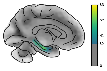
4. Advanced options
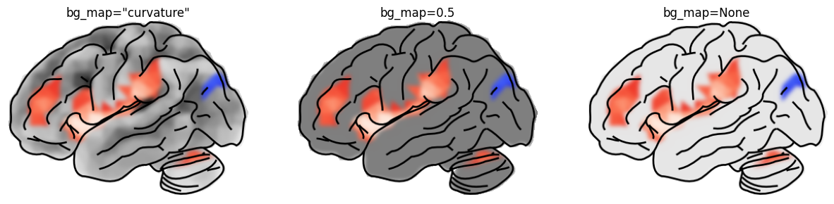
The bg_map parameter controls the underlay:
| value | effect |
|---|---|
"curvature" (default) | signed curvature — highlights gyri/sulci |
a float, e.g. 0.5 | uniform grey |
None | no background (white) |
fig, (ax1, ax2, ax3) = plt.subplots(
    1, 3,
    figsize=(15, 5),
    subplot_kw={"projection": "3d"},
)

for ax, bg, label in [
    (ax1, "curvature", 'bg_map="curvature"'),
    (ax2, 0.5, "bg_map=0.5"),
    (ax3, 0.1, "bg_map=None"),
]:
    plot_brain(
        statmap,
        bg_map=bg,
        threshold=0.5,
        axes=ax,
        colorbar=False,
        title=label,
        cmap='blue_red',
    )

plt.tight_layout()
plt.show()
/var/folders/rc/b4064_3d4dj60wt9y_447fyr0000gn/T/ipykernel_55088/3448203987.py:22: UserWarning: This figure includes Axes that are not compatible with tight_layout, so results might be incorrect.
plt.tight_layout()
background="transparent" turns the white canvas transparent (useful for
compositing into posters or slides). Only two values are allowed:
"white" (default) and "transparent".
Note: this feature is under development and may not work as expected.
fig, (ax1, ax2) = plt.subplots(
    1, 2,
    figsize=(15, 5),
    subplot_kw={"projection": "3d"},
)

# set plot canvas background to black
fig.patch.set_facecolor('black')


plot_brain(statmap, background="transparent", axes=ax1, colorbar=False)
plot_brain(statmap, background="white", axes=ax2, colorbar=False)
plt.show()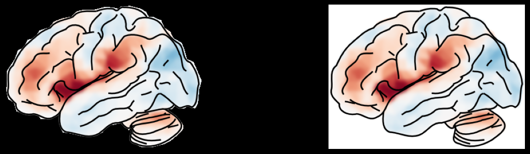
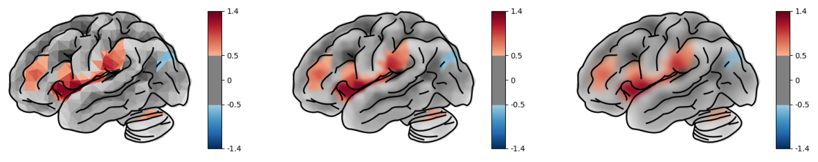
We can also costume or hide the overlay contours.
fig, (ax1, ax2, ax3, ax4) = plt.subplots(
    1, 4,
    figsize=(15, 5),
    subplot_kw={"projection": "3d"},
)

plot_brain(statmap, threshold=0.5, axes=ax1, overlay=None)
plot_brain(statmap, threshold=0.5, axes=ax2, overlay_linewidth=0.5)
plot_brain(statmap, threshold=0.5, axes=ax3, overlay_linewidth=1)
plot_brain(statmap, threshold=0.5, axes=ax4, overlay_linewidth=2)
plt.tight_layout()
plt.show()
/var/folders/rc/b4064_3d4dj60wt9y_447fyr0000gn/T/ipykernel_55088/3106201497.py:11: UserWarning: This figure includes Axes that are not compatible with tight_layout, so results might be incorrect.
plt.tight_layout()
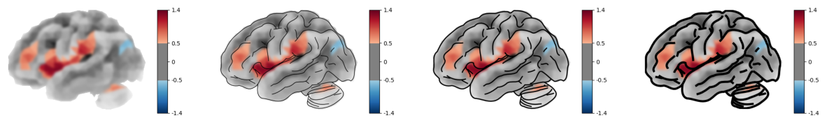
post_blur (default 3 px) applies a light Gaussian blur to the brain
rendering before the SVG overlay is composited. This softens the
polygon edges. Set to 0 to disable.
In most cases the default blur is fine.
fig, (ax1, ax2, ax3) = plt.subplots(
    1, 3,
    figsize=(15, 5),
    subplot_kw={"projection": "3d"},
)

plot_brain(statmap, threshold=0.5, axes=ax1, post_blur=0)
plot_brain(statmap, threshold=0.5, axes=ax2, post_blur=3)
plot_brain(statmap, threshold=0.5, axes=ax3, post_blur=6)
plt.tight_layout()
plt.show()
/var/folders/rc/b4064_3d4dj60wt9y_447fyr0000gn/T/ipykernel_55088/2637619677.py:10: UserWarning: This figure includes Axes that are not compatible with tight_layout, so results might be incorrect.
plt.tight_layout()
5. Saving to file
Use output_file to write the figure directly (any format matplotlib
supports: png, pdf, svg, ...).
plot_brain(
    statmap,
    threshold=0.5,
    hemi="right",
    view="medial",
    title="Right medial",
    output_file="/tmp/quickbrain_demo.png",
    overlay=None,
)
print("Saved to /tmp/quickbrain_demo.png")
Saved to /tmp/quickbrain_demo.png