Abstract
Attractor dynamics are a hallmark of many complex systems, including the brain. Understanding how such self-organizing dynamics emerge from first principles is crucial for advancing our understanding of neuronal computations and the design of artificial intelligence systems. Here we formalize how attractor networks emerge from the free energy principle applied to a universal partitioning of random dynamical systems. Our approach obviates the need for explicitly imposed learning and inference rules and identifies emergent, but efficient and biologically plausible inference and learning dynamics for such self-organizing systems. These result in a collective, multi-level Bayesian active inference process. Attractors on the free energy landscape encode prior beliefs; inference integrates sensory data into posterior beliefs; and learning fine-tunes couplings to minimize long-term surprise. Analytically and via simulations, we establish that the proposed networks favor approximately orthogonalized attractor representations, a consequence of simultaneously optimizing predictive accuracy and model complexity. These attractors efficiently span the input subspace, enhancing generalization and the mutual information between hidden causes and observable effects. Furthermore, while random data presentation leads to symmetric and sparse couplings, sequential data fosters asymmetric couplings and non-equilibrium steady-state dynamics, offering a natural generalization of conventional Boltzmann Machines. Our findings offer a unifying theory of self-organizing attractor networks, providing novel insights for AI and neuroscience.
Key Points
Attractor networks are derived from the Free Energy Principle (FEP) applied to a universal partitioning of random dynamical systems.
This approach yields emergent, biologically plausible inference and learning dynamics, forming a multi-level Bayesian active inference process.
The networks favor approximately orthogonalized attractor representations, optimizing predictive accuracy and model complexity.
Sequential data presentation leads to asymmetric couplings and non-equilibrium steady-state dynamics, generalizing conventional Boltzmann Machines.
Simulations demonstrate orthogonal basis formation, generalization, sequence learning, scalability and resistance to catastrophic forgetting.
Graphical Abstract

Introduction
From whirlpools and bird flocks to neuronal and social networks, countless natural systems can be characterized by dynamics organized around attractor states Haken, 1978. Such systems can be decomposed into a collection of - less or more complex - building blocks or “particles” (e.g. water molecules, birds, neurons, or people), which are coupled through local interactions. Attractors are an emergent consequence of the collective dynamics of the system, arising from these local interactions, without any individual particles exerting global control.
Attractors are a key concept in dynamical systems theory, defined as a set of states in the state space of the system to which nearby trajectories converge Guckenheimer et al., 1984. Geometrically, the simplest attractors are fixed points and limit cycles (representing periodic oscillations). However, the concept extends to more complex structures like strange attractors associated with chaotic behavior, as well as phenomena arising in stochastic or non-equilibrium settings, such as probability distributions over states (stochastic attractors), transient states reflecting past dynamics (ghost attractors or attractor ruins), and trajectories that cycle through sequences of unstable states (sequential attractors or heteroclinic cycles). Artificial attractor neural networks Amit, 1989 represent a class of recurrent neural networks specifically designed to leverage attractor dynamics. While the specific forms and behaviors of these networks are heavily influenced by the chosen inference and learning rules, self-organization is a key feature of all variants, as the stable states emerge from the interactions between network elements without explicit external coordination. This property makes them particularly relevant as models for self-organizing biological systems, including the brain. It is clear that the brain is also a complex attractor network. Attractor dynamics have long been proposed to play a significant role in information integration at the circuit level Freeman, 1987Amit, 1989Deco & Rolls, 2003Nartallo-Kaluarachchi et al., 2025 (Tsodyks (1999)) and have become established models for canonical brain circuits involved in motor control, sensory amplification, motion integration, evidence integration, memory, decision-making, and spatial navigation (see Khona & Fiete (2022) for a review). For instance, the activity of head direction cells - neurons that fire in a direction-dependent manner - are known to arise from a circular attractor state, produced by a so-called ring attractor network Zhang, 1996. Multi- and metastable attractor dynamics have also been proposed to extend to the meso- and macro-scales Rolls, 2009, “accommodating the coordination of heterogeneous elements” Kelso, 2012, rendering attractor dynamics an overarching computational mechanism across different scales of brain function. The brain, as an instance of complex attractor networks, showcases not only the computational capabilities of this network architecture but also its ability to emerge and evolve through self-organization.
When discussing self-organization in attractor networks, we will differentiate two distinct levels. First, we can talk about operational self-organization: the capacity of a pre-formed network to settle into attractor states during its operation. This however does not encompass the network’s ability to “build itself” – to emerge from simple, local interactions without explicit programming or global control, and to adaptively evolve its structure and function through learning. This latter level of self-organization is what we will refer to as adaptive self-organization. Architectures capable of adaptive self-organization would mirror the nervous system’s capacity to not just function as an attractor network, but to become - and remain - one through a self-directed process of development and learning. Further, adaptive self-organization would also be a highly desirable property for robotics and artificial intelligence systems, not only boosting their robustness and adaptability by means of continuous learning, but potentially leading to systems that can increase their complexity and capabilities organically over time (e.g. developmental robotics). Therefore, characterizing adaptive self-organization in attractor networks is vital for advancing our understanding of the brain and for creating more autonomous, adaptive, brain-inspired AI systems.
The Free Energy Principle (FEP) offers a general framework to study self-organization to non-equilibrium steady states as Bayesian inference (a.k.a., active inference). The FEP has been pivotal in connecting the dynamics of complex self-organizing systems with computational and inferential processes, especially within the realms of brain function Friston et al., 2023Friston & Ao, 2012Palacios et al., 2020. The FEP posits that any ‘thing’ - in order to exist for an extended period of time - must maintain conditional independence from its environment. This entails a specific sparsely coupled structure of the system, referred to as a particular partition, that divides the system into internal, external, and boundary (sensory and active) states (see Figure 2A). It can be shown that maintaining this sparse coupling is equivalent to executing an inference process, where internal states deduce the causes of sensory inputs by minimizing variational free energy (see Friston et al. (2023) or Friston et al., 2023 for a formal treatment).
Here, we describe the specific class of adaptive self-organizing attractor networks that emerge directly from the FEP, without the need for explicitly imposed learning or inference rules (Figure 1). First, we show that a hierarchical formulation of particular partitions - a concept that is applicable to any complex dynamical system - can give rise to systems that have the same functional form as well-known artificial attractor network architectures. Second, we show that minimizing variational free energy (VFE) with regard to the internal states of such systems yields a Boltzmann Machine-like stochastic update mechanism, with continuous-state stochastic Hopfield networks being a special case. Third, we show that minimizing VFE with regard to the internal blanket or boundary states of the system (couplings) induces a generalized predictive coding-based learning process. Crucially, this adaptive process extends beyond simply reinforcing concrete sensory patterns; it learns to span the entire subspace of key patterns by establishing approximately-orthogonalized attractor representations, which the system can then combine during inference. We use simulations to identify the requirements for the emergence of quasi-orthogonal attractors and to illustrate the derived attractor networks’ ability to generalize to unseen data. Finally, we highlight that the derived attractor network can naturally produce sequence-attractors (if the input data is presented in a clear sequential order) and exemplifies its potential to perform continual learning and to overcome catastrophic forgetting by means of spontaneous activity. We conclude by discussing testable predictions of our framework, and exploring the broader implications of these findings for both natural and artificial intelligence systems.

Figure 1:Overview of the framework. Starting from universal and parsimonious structural assumptions (deep particular partition), variational free energy minimization under the Free Energy Principle (FEP) gives rise to emergent dynamics at multiple scales: local stochastic inference and learning rules that guide the update of internal states and the couplings between them, self-organizing attractor dynamics at the macroscale, and — at the computational level — Bayesian inference, approximately orthogonal attractor representations of latent external causes, and sequence learning capabilities.
Main Results
Background: particular partitions and the free energy principle
Our effort to characterize self-organizing attractor networks calls for an individuation of ‘self’ from nonself. Particular partitions, a concept that is at the core of the Free Energy Principle (FEP) Friston et al., 2022Friston et al., 2023Friston & Ao, 2012Palacios et al., 2020, is a natural way to formalize this individuation. As a toy intuition, one can think of a recurrent neural assembly (internal states) interacting with incoming sensory drives and outgoing action channels (blanket states), while latent external causes remain hidden. The blanket states mediate all interactions, which is exactly the structure needed for inference to be well-defined. A particular partition is a partition that divides the states of a system into a particle or ‘thing’ and its external states , based on their sparse coupling:
where , , , and are the external, internal, sensory, and active states of the particle, respectively. The fluctuations are assumed to be mutually independent. The particular states , , and are coupled to each other with particular flow dependencies; namely, external states can only influence themselves and sensory states, while internal states can only influence themselves and active states (see Figure 2A). It can be shown that these coupling constraints mean that external and internal paths are statistically independent, when conditioned on and , often referred to as the Markov blanket Friston et al., 2022:
At an intuitive level, considering particular partitioning as a “universal partitioning” means that any persistent random dynamical system can be described with (possibly nested) interfaces that separate what is inferred from what is inferred about. In this view, Markov blankets are not ad hoc modeling devices, but the minimal bookkeeping needed to explain how local interactions can support stable, self-organizing inference across scales.
As shown by Friston et al. (2023), such a particle, in order to persist for an extended period of time, will necessarily have to maintain this conditional independence structure, a behavior that is equivalent to an inference process in which internal states infer external states through the blanket states (i.e., sensory and active states) by minimizing free energy Friston et al., 2009Friston, 2010Friston et al., 2023:
where is the variational free energy (VFE):
with being a variational density over the external states that is parameterized by the internal states and being the joint probability distribution of the sensory, active and external states, a.k.a. the generative model Friston et al., 2016.

Figure 2:Deep Particular Partitions.
A Schematic illustration of a particular partition of a system into internal () and external states (), separated by a Markov blanket consisting of sensory states () and active states (). The tuple is called a particle. A particle, in order to persist for an extended period of time, will necessarily have to maintain its Markov blanket, a behavior that is equivalent to an inference process in which internal states infer external states through the blanket states. The resulting self-organization of internal states corresponds to perception, while actions link the internal states back to the external states.
B The internal states can be arbitrarily complex. Without loss of generality, we can consider that the macro-scale can be decomposed into set of overlapping micro-scale subparticles (), so that the internal state of subparticle can be an external state from the perspective of another subparticle . Some, or all subparticles can be connected to the macro-scale external state , through the macro-scale Markov blanket, giving a decomposition of the original boundary states into and . The subparticles are connected to each other by the micro-scale boundary states and . Note that this notation considers the point-of-view of the -th subparticle. Taking the perspective of the -th subparticle, we can see that and . While the figure depicts the simplest case of two nested partitions, the same scheme can be applied recursively to any number of (possibly nested) subparticles and any coupling structure amongst them.
Deep particular partitions and subparticles
Particular partitions provide a universal description of complex systems, in the sense that the internal states behave as if they are inferring the external states under a generative model; i.e., a ‘black box’ inference process (or computation), which can be arbitrarily complex. At the same time, the concept of particular partitions speaks to a recursive composition of ensembles (of things) at increasingly higher spatiotemporal scales Friston, 2019Palacios et al., 2020Clark, 2017, which yields a natural way to resolve the internal complexity of . Partitioning the “macro-scale” particle into multiple, overlapping “micro-scale” subparticles - that themselves are particular partitions - we can unfold the complexity of the macro-scale particle to an arbitrary degree. As subparticles can be nested arbitrarily deep - yielding a hierarchical generative model - we refer to such a partitioning as a deep particular partition.
As illustrated in Figure 2B, each subparticle has internal states , and the coupling between any two subparticles and is mediated by micro-scale boundary states: sensory states (representing the sensory information in coming from ) and active states (representing the action of on ). The boundary states of subparticles naturally overlap; the sensory state of a subparticle is the active state of and vice versa, i.e. and . This also means that, at the micro-scale, the internal state of a subparticle is part of the external states for another subparticle in . Accordingly, the internal state of a subparticle is conditionally independent of any other internal states with , given the blanket states of the subparticles:
Note that this definition embraces sparse couplings across subparticles, as and may be empty for a given (no direct connection between the two subparticles), but we require the subparticles to yield a complete coverage of : .
The emergence of attractor neural networks from deep particular partitions
Next, we establish a prototypical mathematical parametrization for an arbitrary deep particular partition, shown on Figure 3, with the aim of demonstrating that such complex, sparsely coupled random dynamical systems can give rise to artificial attractor neural networks.
![Parametrization of subparticles in a deep particular partition.
The internal state \sigma_i of subparticle \pi_i follows a continuous Bernoulli distribution, (a.k.a. a truncated exponential distribution supported on the interval [-1, +1] \subset \mathbb{R}, see ), with a prior “bias” b_i that can be interpreted as a priori log-odds evidence for an event (stemming from a macro-scale sensory input s_{i} - not shown, or from the internal dynamics of \sigma_i itself, e.g. internal sequence dynamics).
The state \sigma_i is coupled to the internal state of another subparticle \sigma_j through the micro-scale boundary states s_{ij} and a_{ij}. The boundary states simply apply a deterministic scaling to their respective \sigma state, with a weight (J_{ij}) implemented by a Dirac delta function shifted by J_{ij} (i.e. we deal with conservative subparticles, in the sense of ). The state \sigma_i is influenced by its sensory input s_i in a way that s_i gets integrated into its internal bias, updating the level of evidence for the represented event.](/fep-attractor-network/build/parametrization-0779151e94595a5fc00d9c8868075d8d.webp)
Figure 3:Parametrization of subparticles in a deep particular partition.
The internal state of subparticle follows a continuous Bernoulli distribution, (a.k.a. a truncated exponential distribution supported on the interval , see Appendix 1), with a prior “bias” that can be interpreted as a priori log-odds evidence for an event (stemming from a macro-scale sensory input - not shown, or from the internal dynamics of itself, e.g. internal sequence dynamics).
The state is coupled to the internal state of another subparticle through the micro-scale boundary states and . The boundary states simply apply a deterministic scaling to their respective state, with a weight () implemented by a Dirac delta function shifted by (i.e. we deal with conservative subparticles, in the sense of Friston et al. (2023)). The state is influenced by its sensory input in a way that gets integrated into its internal bias, updating the level of evidence for the represented event.
In our example parametrization, we assume that the internal states of subparticles in a complex particular partition are continuous Bernoulli states (also known as a truncated exponential distribution, see Appendix 1 for details), denoted by :
Here, , and represents an a priori bias (e.g. the level of prior log-odds evidence for an event) in Figure 3. Zero bias represents a flat prior (uniform distribution over [-1,1]), while positive or negative biases represent evidence for or against an event, respectively. The above probability is defined up to a normalization constant, . See Appendix 2 for details.
Note that the assumption of continuous Bernoulli distribution is very parsimonious; it emerges directly from FEP through as the constrained maximum entropy solution to a single constraint on mean, plus finite support Ramstead et al., 2023.
Next, we define the conditional probabilities of the sensory and active states, creating the boundary between two subparticles and : and , where is the Dirac delta function and is a weight matrix. The elements contains the weights of the coupling matrix (see Appendix 3).
Expressed as PDFs:
The choice of this deterministic parametrization means that we introduce the assumption of the subparticles being conservative particles, as defined in Friston et al. (2023).
To close the loop, we define how the internal state depends on its sensory input . We assume the sensory input simply adds to the prior bias :
With the continuous Bernoulli distribution, this simply means that the sensory evidence adds to (or subtracts from) the prior belief .
We now write up the direct conditional probability describing given , marginalizing out the sensory and active states:
More generally, when sub-particle receives sensory input from all other sub-particles, the combined evidence at node is:
The local conditional is a continuous Bernoulli with parameter , and its expected value is , the Langevin function. This local evidence form is the basis for the inference and learning rules derived in the following sections: they follow from VFE minimization at each node using only , and depend on the full (potentially asymmetric) coupling matrix . The global consequences of the coupling structure — including the stationary distribution and non-equilibrium steady-state dynamics — are discussed in .
Inference
So far our derivation relied only on the sparsely coupled structure of the system (deep particular partition), but did not utilize the free energy principle itself. We now invoke the FEP to derive how each node updates its state. From the perspective of node , the local variational free energy is (see eq. (4)):
where is the variational density over , its entropy, and is the total evidence at node (eq. (11)). For the continuous Bernoulli likelihood, (up to a constant, where is the log-partition function), giving:
Minimizing over all normalized densities supported on yields (see Appendix 6 for the full derivation via accuracy–complexity decomposition):
That is, the optimal variational density is the continuous Bernoulli with parameter , recovering the local posterior family that can be derived from the constrained maximum entropy construction Ramstead et al., 2023. The expected value under this optimal posterior gives the inference rule:
This derivation is purely local: it uses only the conditional at each node and does not require the global joint distribution (eq. (24)). In the case of symmetric couplings, it reduces to the familiar Boltzmann-style update rule of a continuous-state stochastic Hopfield network. The Langevin sigmoid arises naturally from the continuous Bernoulli parameterization, extending the standard deterministic gradient descent on the energy landscape to a full probabilistic framework (see Appendix 6). The resulting stochastic dynamics represents a local approximate Bayesian inference, where each node balances prior information () with evidence from neighboring nodes (). As we show below, this inherent stochasticity allows the network to escape local energy minima — consistent with MCMC methods — thereby enabling macro-scale Bayesian inference.
Learning
At optimum, would match , causing the VFE’s derivative to vanish. Learning happens, when there is a systematic change in the prior bias that counteracts the update process. This can correspond, for instance, to an external input (e.g. sensory signal representing increased evidence for an external event), but also as the result of the possibly complex internal dynamics of a subparticle (e.g. internal sequence dynamics or memory retrieval). In this case, a subparticle can take use of another (slower) process, to decrease local VFE: it can change the way its action states are generated; and rely on its vicarious effects on sensory signals. In our parametrization, this can be achieved by changing the coupling strength corresponding to the action states. Of note, while changing corresponds to a change in action-generation at the local level of the subparticle (micro-scale), at the macro-scale, it can be considered as a change in the whole system’s generative model.
Using the local VFE from eq. (12) with a point-mass (sample-based) estimate for , the reduced objective for the coupling gradient is:
where is the total evidence at node . A perturbation produces , and by the chain rule:
Gradient descent on yields:
This learning resembles the family of “Hebbian / anti-Hebbian” or “contrastive” learning rules and it explicitly implements predictive coding (akin to prospective configuration Song et al., 2024Millidge et al., 2022). However, as opposed to e.g. contrastive divergence (a common method for training certain types of Boltzmann machines, Hinton (2002)), it does not require to contrast longer averages of separate “clamped” (fixed inputs) and “free” (free running) phases, but rather uses the instantaneous correlation between presynaptic and postsynaptic activation to update the weight, lending a high degree of scalability for this architecture. As we demonstrate below with Simulation Notebook 1-4, this learning rule converges to symmetric weights (akin to a classical stochastic continuous-state Hopfield network), if input data is presented in random order and long epochs. At the same time, if data is presented in rapidly changing fixed sequences (Simulation Notebook 3), the learning rule results in temporal predictive coding and learns asymmetric weights, akin to Millidge et al., 2024. As discussed above, in this case the symmetric component of encodes fixed-point attractors and the probability flux induced by the antisymmetric component results in sequence dynamics (conservative solenoidal flow), without altering the steady state of the system.
Other key features of this rule are: (i) its resemblance to Sanger’s rule Sanger, 1989 - an online algorithm for principal component analysis - and (ii) the analogy of its anti-Hebbian component to unlearning (“remotion”) processes in “dreaming attractor networks” Hopfield et al., 1983Plakhov, n.d.Dotsenko & Tirozzi, 1991Fachechi et al., 2019, which serve to eliminate spurious system attractors. Such networks can effectively approximate Kanter-Sompolinsky projector neural networks Personnaz et al., 1985Kanter & Sompolinsky, 1987, characterized by orthogonal attractor states and maximal memory capacity. These parallels suggest that the derived free energy minimizing learning rule will promote the development of approximately orthogonal attractor states. We motivate this theoretically and demonstrate it with simulations in the subsequent sections. In biological terms, the first term of eq. (18) corresponds to correlation-dependent potentiation, while the second term implements a decorrelating, predictive-error-like correction that counterbalances runaway reinforcement. This places the rule in the algorithmic family of Hebbian/anti-Hebbian and homeostatically stabilized plasticity motifs, while we do not claim a one-to-one mapping to any single microcircuit mechanism. In other words, the derivation is normative (from free-energy minimization), and biological plausibility is asserted at the level of local computable updates and observed qualitative motifs.
Emergence of approximately orthogonal attractors
Under the FEP, learning not only aims to maximize accuracy but also minimizes complexity (12), leading to parsimonious internal generative models (encoded in the weights and biases ) that offer efficient representations of environmental regularities. A generative model is considered more complex (and less efficient) if its internal representations, specifically its attractor states - which loosely correspond to the modes of - are highly correlated or statistically dependent. Such correlations imply redundancy, as distinct attractors would not be encoding unique, independent features of the input space. Our learning rule (eq. (18)) - by minimizing micro-scale VFE - inherently also minimizes the complexity term , which regularizes the inferred state to be close to the node’s current prior . This not only induces sparsity in the coupling matrix, but - as we motivate below - also penalizes overlapping attractor representations and favours orthogonal representations. Hebbian learning - in itself - can not implement such a behavior; as it simply aims to store the current pattern by strengthening connections between co-active nodes. This has to be counter-balanced by the anti-Hebbian term, that subtracts the variance that is already explained out by the network’s predictions.
To illustrate how this dynamic gives rise to efficient, (approximately) orthogonal representations of the external states, suppose the network has already learned a pattern , whose neural representation is the attractor and associated weights . When a new pattern is presented that is correlated with , the network’s prediction for will be . Because inference with converges to and is correlated with , the prediction will capture variance in that is ‘explained’ by . The learning rule updates the weights based only on the unexplained (residual) component of the variance, the prediction error. In other words, approximates the projection of onto the subspace already spanned by . Therefore, the weight update primarily strengthens weights corresponding to the component of that is orthogonal to . Thus, the learning effectively encodes this residual, , ensuring that the new attractor components being formed tend to be orthogonal to those already established. As we demonstrate in the next section with Simulation Notebook 1-2, repeated application of this rule during learning progressively decorrelates the neural activities associated with different patterns, leading to approximately orthogonal attractor states. This process is analogous to online orthogonalization procedures (e.g., Sanger’s rule for PCA Sanger, 1989), as well as the converge of Plakhov (n.d.)’s unlearning rule to the projector (or pseudo-inverse) matrix of stored patterns Fachechi et al., 2019. As a result, free energy minimizing attractor networks yield a powerful stochastic approximation of the “projector networks” of Personnaz et al. (1985), Kanter & Sompolinsky (1987), which offer maximal memory capacity and retrieval without errors.
While orthogonality enhances representational efficiency, it raises the question of how the network retrieves the original patterns from these (approximately) orthogonalized representations - a key requirement to function as associative memory. As discussed next, stochastic dynamics enable the network to address this by sampling from a posterior that combines these orthogonal bases.
Stochastic retrieval as macro-scale Bayesian inference
As a consequence of the FEP, the inference process described above - where each subparticle updates its state based on local information (its bias and input ) - can be seen as a form of micro-scale inference, in which the prior - defined by the node’s internal bias, gets updated by the evidence collected from the neighboring subparticles to form the posterior. However, as the whole network itself is also a particular partition (specifically, a deep one), it must also perform Bayesian inference, at the macro-scale. While the above argumentation provides a simple, self-contained proof, the nature of macro-scale inference can be elucidated by using the equivalence of the derived attractor network - in the special case of symmetric couplings - to Boltzmann machines (without hidden units). Namely, the ability of Boltzmann machines to perform macro-scale approximate Bayesian inference through Markov Chain Monte Carlo (MCMC) sampling has been well established in the literature ACKLEY et al., 1985Hinton, 2002.
Let us consider the network’s learned weights (and potentially its baseline biases ) as defining a prior distribution over the collective states :
Now, suppose the network receives external input (evidence) , which manifests as persistent modulations to the biases, such that the total bias is . This evidence can be associated with a likelihood function:
According to Bayes’ theorem, the posterior distribution over the network states given the evidence is :
As expected, this posterior distribution has the same functional form as the network’s equilibrium distribution under the influence of the total biases . Thus, the stochastic update rule derived from minimizing local VFE (eq. (12)) effectively performs Markov Chain Monte Carlo (MCMC) sampling - specifically Gibbs sampling - from the joint posterior distribution defined by the current VFE landscape. In the presence of evidence , the network dynamics therefore sample from the posterior distribution . The significance of the stochasticity becomes apparent when considering the network’s behavior over time. The time-averaged state converges to the expected value under the posterior distribution:
Noise or stochasticity allows the system to explore the posterior landscape, escaping local minima inherited from the prior if they conflict with the evidence, and potentially mixing between multiple attractors that are compatible with the evidence. The resulting average activity thus represents a Bayesian integration of the prior knowledge encoded in the weights and the current evidence encoded in the biases. This contrasts sharply with deterministic dynamics, which would merely settle into a single (potentially suboptimal) attractor within the posterior landscape.
Furthermore, if the learning process shapes the prior to have less redundant (e.g., more orthogonal) attractors, this parsimonious structure of the prior naturally contributes to a less redundant posterior distribution . When the prior belief structure is efficient and its modes are distinct, the posterior modes formed by integrating evidence are also less likely to be ambiguous or highly overlapping. This leads to more robust and interpretable inference, as the network can more clearly distinguish between different explanations for the sensory data.
With this, the loop is closed. The stochastic attractor network emerging from the FEP framework (summarized on Figure 4A) naturally implements macro-scale Bayesian inference through its collective sampling dynamics, providing a robust mechanism for integrating prior beliefs with incoming sensory evidence — as demonstrated concretely on the face recognition task (Figure 7F), where the network recovers face identity from heavily corrupted input by combining sensory evidence with attractor-based priors. This reveals the potential for a deep recursive application of the Free Energy Principle: the emergent collective behavior of the entire network, formed by interacting subparticles each minimizing their local free energy, recapitulates the inferential dynamics of a single, macro-scale particle. This recursion could extend to arbitrary depths, giving rise to a hierarchy of nested particular partitions and multiple emergent levels of description, each level performing Bayesian active inference according to the same fundamental principles.

Figure 4:Free energy minimizing, adaptively self-organizing attractor network
A Schematic of the network illustrating inference and learning processes. Inference and learning are two faces of the same process: minimizing local variational free energy (VFE), leading to dissipative dynamics and approximately orthogonal attractors.
B A demonstrative simulated example (Simulation Notebook 1) of the network’s attractors forming an orthogonal basis of the input data. Training can be performed by introducing the training data (top left) through the biases of the network. In this example, the input data consists of two correlated patterns (Pearson’s r = 0.77). During repeated updates, micro-scale (local, node-level) VFE minimization implements a simultaneous learning and inference process, which leads to approximate macro-scale (network-level) free energy minimization (bottom graph). The resulting network does not simply store the input data as attractors, but it stores approximately orthogonalized varieties of it (top right, Pearson’s r = -0.19).
C When the trained network is introduced a noisy version of one of the training patterns (left), it is internally handled as the Likelihood function, and the network performs irreversible Markov-Chain Monte-Carlo (MCMC) sampling of the posterior distribution, given the priors defined by the network’s attractors (top right), which can be understood as a retrieval process.
D Thanks to its orthogonal attractor representation, the network is able to generalize to new patterns - as long as they are sampled from the sub-space spanned by the attractors - by combining the quasi-orthogonal attractor states (bottom right) by multistable stochastic dynamics during the MCMC sampling.
Non-equilibrium steady state
We now turn from the local update rules to the global steady-state behaviour of the network. The coupling matrix can always be decomposed as , where is symmetric and is antisymmetric. We consider these two components in turn.
Symmetric couplings and the Boltzmann-like stationary distribution. When the learning rule (eq. (18)) is driven by randomly ordered input patterns, it converges to approximately symmetric weights (). In this case the pairwise conditionals are symmetric in their coupling terms (), and the conditional independence structure of the Markov blanket states , Hipólito et al., 2021 allows us to factorise the global joint as . Since , one obtains:
which, for symmetric , yields the Boltzmann form:
with (and ). This is the functional form of a stochastic continuous-state Hopfield network (a specific type of Boltzmann machine), with regions of high probability density constituting stochastic attractors.
Asymmetric couplings and self-solenoidization. When data arrives in fixed sequences, the learning rule additionally develops an antisymmetric component . The simple factorisation argument above no longer applies, because directed couplings break the symmetry . Nevertheless, we argue that the Boltzmann-like stationary distribution (eq. (24)) is approximately preserved, with solenoidal flows on top.
The key intuition is that self-orthogonalization provides the missing link. Because VFE-driven learning pushes attractor representations toward approximate orthogonality, the antisymmetric coupling component — which encodes directed transitions between attractors — acts predominantly along the iso-energy contours of the landscape defined by . Any component of the antisymmetric flow that were to act across iso-energy contours would imply shared information between attractors; but precisely this shared information is progressively absorbed into the symmetric part by the residual (anti-Hebbian) learning rule. In other words, the same mechanism that orthogonalizes attractors also ensures that the inter-attractor transition flows are approximately tangential to the energy landscape — i.e., approximately solenoidal.
Under this condition, the network dynamics decompose into two complementary components: (i) Dissipative (gradient) flow, driven by : descends the free energy landscape, pulling states toward attractor basins. Responsible for pattern storage and retrieval, and (ii) Solenoidal (rotational) flow, driven by : generates probability currents along iso-energy contours — analogous to a ball circling within a bowl rather than simply rolling to the bottom.
Thus the dynamics induced by and will approximately map to the generalized Helmholtz-Ao decomposition of the network dynamics (see also Appendix 5 and Friston et al., 2023Ao, 2004Xing, 2010). Because the solenoidal term transports probability mass along iso-energy surfaces without altering the potential, the stationary distribution retains the Boltzmann-like form of eq. (24), while detailed balance is broken by persistent probability currents.
The practical consequences are twofold. First, directed sequence dynamics (heteroclinic chains) emerge naturally from the solenoidal component, enabling the network to traverse stored patterns in a learned temporal order — as demonstrated in Simulation 3. Second, the non-reversible currents can transport probability mass between attractor basins without climbing energy barriers, potentially accelerating mixing relative to the reversible (symmetric-coupling) case Ao, 2004Xing, 2010. A rigorous characterization of the relationship between attractor orthogonality and the divergence-free condition — and of the resulting mixing-time improvements — is an important direction for future work. As a first step, in the present work we perform simulations (Simulation Notebook 3) to confirm that the key phenomenology — stable attractors with directed inter-attractor transitions — is robustly observed.
In silico demonstrations
We illustrate key features of the proposed framework with computer simulations. All simulations are based on python implementations of the network, available at https://
Simulation 1: demonstration of orthogonal basis formation, macro-scale free energy minimization and Bayesian inference
In Simulation Notebook 1, we construct a network with 25 subparticles (representing 5x5 images) and train it with 2 different, but correlated images (Pearson’s r = 0.77, see Figure 4B), with a precision of 0.1 and a learning rate of 0.01 (see next simulation for parameter-dependence). The training phase consisted of 500 epochs, each showing a randomly selected pattern from the training set through 10 time steps of simultaneous inference and learning. As shown on Figure 4B, local, micro-scale VFE minimization performed by the simultaneous inference and learning process leads to a macro-scale free energy minimization. Next, we obtained the attractor states corresponding to the input patterns by means of deterministic inference (updating with the expected value, instead of sampling from the distribution, akin to a vanilla Hopfield network). As predicted by theory, the attractor states were not simple replicas of the input patterns, but approximately orthogonalized versions of them, displaying a correlation coefficient of r=-0.19. Next, we demonstrated that the network (with stochastic inference) is not only able to retrieve the input patterns from noisy variations of them (fig. Figure 4C), but also generalizes well to reconstruct a third pattern, by combining its quasi-orthogonal attractor states (fig. Figure 4D). Note that this simulation only aimed to demonstrate some of the key features of the proposed architecture, and a comprehensive evaluation of the network’s performance, and its dependency on the parameters is presented in the next simulation.
Simulation 2: systematic evaluation of learning regimes
In Simulation Notebook 2, we trained the network on 10 images of handwritten digits (a single example of each of the 10 digits from 0 to 9, 8x8 pixels each, as distributed with scikit-learn, see Figure 5C, upper row). The remaining 1787 images were unseen in the training phase and only used as a test set, in a one-shot learning fashion. The network was trained with a fixed learning rate of 0.01, through 5000 epochs, each consisting of 10 time steps with the same, randomly selected pattern from the training set of 10 images, while performing simultaneous inference and learning. We evaluated the effect of the inverse temperature parameter (i.e. precision) and the strength of evidence during training, i.e. the magnitude of the bias changes . The precision parameter was varied with 19 values between 0.01 and 1, and the strength of evidence during training varied by changing the magnitude of the biases from 1 to 20, with increments of 1. The training patterns were first preprocessed by squaring the pixel values (to enhance contrast) and normalizing each image to have zero mean and unit variance. We performed a total of 380 runs, varying these parameters in a grid-search fashion. All cases were evaluated in terms of (i) stochastic (Bayesian) pattern retrieval from noisy variations of the training images; and (ii) one-shot generalization to reconstruct unseen handwritten digit examples. In both types of evaluation, the network was presented a noisy variant of a randomly selected (training or test) image through its biases. The noisy patterns were generated by adding Gaussian noise with a standard deviation of 1 to the pixel values of the training images (see “Examples” in Figure 5B C and D). The network’s response was obtained by averaging 100 time steps of stochastic inference. The performance was quantified as the improvement in the proportion of variance in the original target pattern (without noise) explained by the network’s response, compared to that explained by the noisy input pattern. Both for retrieval and generalization, this approach was repeated 100 times, with a randomly sampled image from the training (10 images) and test set (1787 images), respectively. The median improvement across these 100 repetition was used as the primary performance metric. The retrieval and 1-shot generalization performance of models trained with different and parameters is shown on Figure 5A, top row). We found that, while retrieval of a noisy training pattern was best with precision values between 0.1 and 0.5, generalization to new data preferred lower precision during learning (<0.1), i.e. more stochastic dynamics. Furthermore, in all simulation cases, we seeded the networks with the original test patterns and obtained the corresponding attractor states, by means of deterministic inference. We then computed the pairwise correlation and dot product between the attractor states. The dot product was converted to degrees. Orthogonality was finally quantified by the mean correlation among attractors and the mean squared deviation from orthogonality (in degrees). To establish a reference value, the same procedure was also repeated for the original patterns (after preprocessing), which displayed a mean correlation a 29.94 degree mean squared deviation from orthogonality. Attractor orthogonality and the number of attractors for each simulation case is shown on Figure 5A, bottom row. We found that depending on the temperature of the network during the learning phase, the network can be in characteristic regimes of high, low and balanced complexity (Figure 5B). With low temperature (high precision), high model complexity is allowed (“accuracy pumping”) and attractors will tend to exactly match the training data Figure 5C. On the contrary, high temperatures (low precision) result in a single fixed point attractor and reduced recognition performance Figure 5E. However, such networks were found to be able to generalize to new data, suggesting the existence of “soft attractors” (e.g. saddle-like structures) that are not local minima on the free energy landscape, yet affect the steady-state posterior distribution in a non-negligible way (especially with longer mixing-times). A balanced regime Figure 5D can be found with intermediate training precision, where both recognition and 1-shot generalization performance are high (similarly to the “standard regime” of prospective configuration Millidge et al., 2022). This is exactly the regime that promotes attractor orthogonalization, crucial for efficient representation and generalization. The complexity restrictions on these models cause them to re-use the same attractors to represent different patterns (see e.g. the single attractor belonging to the digits 5 and 7 in the example on panel D), which eventually leads to less attractors, with each having more explanatory power, and being approximately orthogonal to each other. Panels C-E on Figure 5 provide examples of network behavior on a handwritten digit task across different regimes, including (i) training data (same in all cases); (ii) fixed-point attractors (obtained with deterministic update); (iii) attractor-orthogonality (polar histogram of the pairwise angles between attractors); (iv) retrieval and 1-shot generalization performance ( between the noisy input pattern and the network output after 100 time steps, for 100 randomly sampled patterns) and (v) illustrative example cases from the recognition and 1-shot generalization tests (noisy input, network output and true pattern).
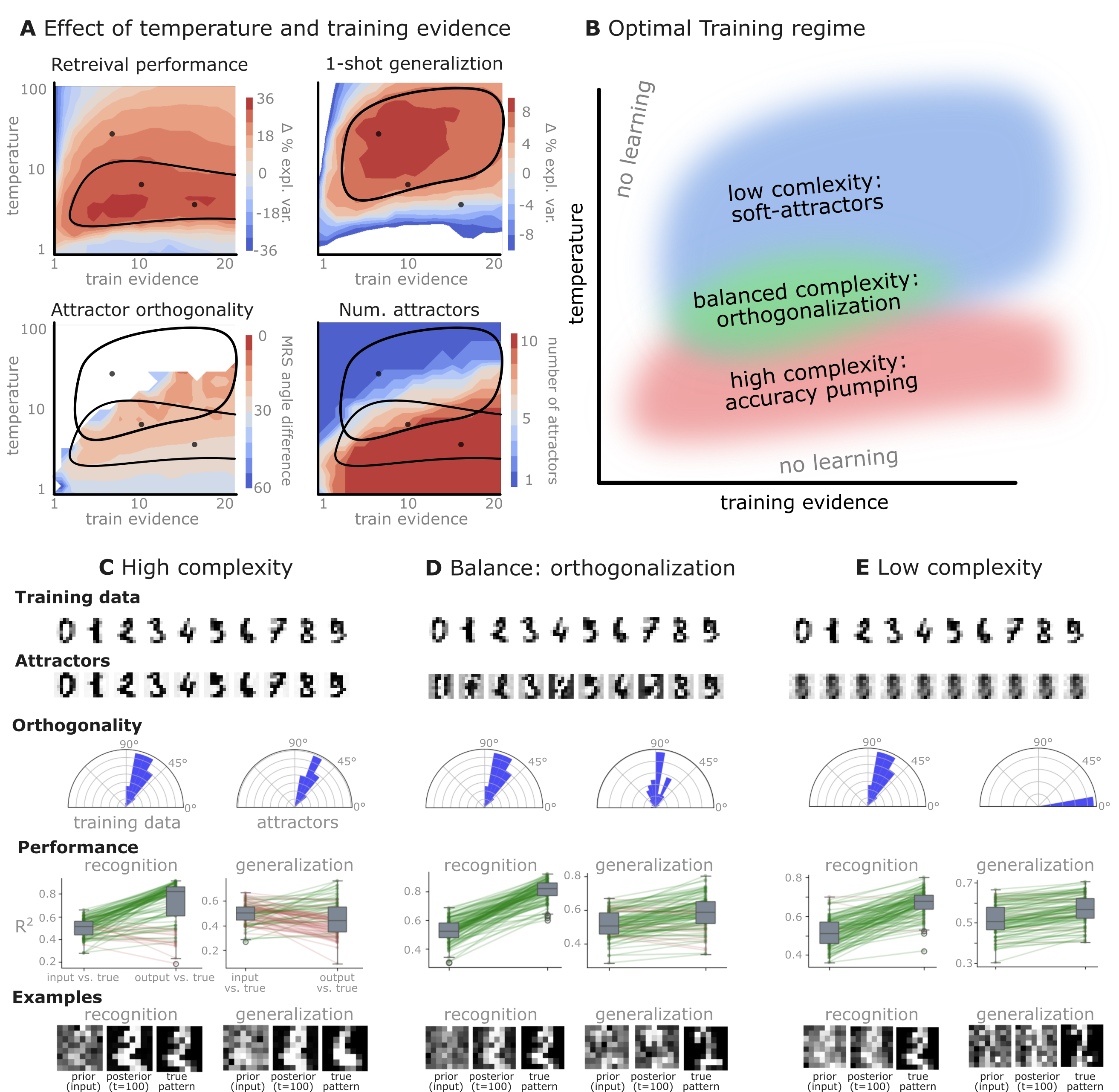
Figure 5:Adaptive self-organization and generalization in a free-energy minimizing attractor network.
Simulation results from training the network on a single, handwritten example for each of the 10 digits (0-9), with variations in training precision and evidence strength to explore different learning regimes (Simulation Notebook 2).
A: Performance landscapes as a function of inference temperature (inverse precision) and training evidence strength (bias magnitude). Retrieval performance (reconstructing noisy variants of the 10 training patterns, top left), one-shot generalization (reconstructing a noisy variants of unseen handwritten digits, top right), attractor orthogonality (mean squared angular difference from 90° indicating higher orthogonality for lower values, bottom left), and the number of attractors (when initialized with the 10 training patterns, bottom right) are shown. Optimal regions (contoured) highlight parameter settings that yield good generalization and highly orthogonal attractors. Contours in the top left and top right highlight the most efficient parameter settings for retrieval and generalization, respectively. Both contours are overlaid on the two bottom plots.
B: Conceptual illustration of training regimes. With low temperature (high precision) high model complexity is allowed (“accuracy pumping”) and attractors will tend to exactly match the training data. On the contrary, high temperatures (low precision) result in a single fixed point attractor and reduced recognition performance. However, such networks will be able to generalize to new data, suggesting the existence of “soft attractors” (e.g. saddle-like structures) that are not local minima on the free energy landscape, yet affect the steady-state posterior distribution in a non-negligible way (especially with longer mixing-times). A balanced regime can be found with intermediate precision during training, where both recognition and generalization performance are high. This is exactly the regime that promotes attractor orthogonalization, crucial for efficient representation and generalization. The complexity restrictions on these models cause them to re-use the same attractors to represent different patterns (see e.g. the single attractor belonging to the digits 5 and 7 in the example on panel D), which eventually leads to approximate orthogonality. Panels C-E provide examples of network behavior on a handwritten digit task across different regimes, including (i) training data (same in all cases); (ii) fixed-point attractors (obtained with deterministic update); (iii) attractor-orthogonality (polar histogram of the pairwise angles between attractors); (iv) retrieval and 1-shot generalization performance ( between the noisy input pattern and the network output after 100 time steps, for 100 randomly sampled patterns) and (v) illustrative example cases from the recognition and 1-shot generalization tests (noisy input, network output and true pattern).
C: High complexity: Attractors are sharp and similar to training data; good recognition, limited generalization.
D: Balanced complexity (orthogonalization): Attractors are distinct and quasi-orthogonal, enabling strong recognition and generalization from noisy inputs. The balanced regime clearly demonstrates the network’s ability to form an orthogonal basis, facilitating effective generalization as predicted by the free-energy minimization framework.
E: Low complexity: There is only a single fixed-point attractor. Recognition performance is lower, but generalization remains considerable.
Simulation 3: demonstration of sequence learning capabilities
In Simulation Notebook 3, we demonstrate the sequence learning capabilities of the proposed architecture. We trained the network on a sequence of 3 handwritten digits (1,2,3), with a fixed order of presentation (), for 2000 epochs, each epoch consisting of a single step (Figure 6A). This rapid presentation of the input sequence forced the network to model the current attractor from the network’s response to the previous pattern, i.e. to establish sequence attractors. The inverse temperature was set to 1 and the learning rate to 0.001 (in a supplementary analysis, we saw a considerable robustness of our results to the choice of these parameters). As shown on Figure 6B, this training approach led to an asymmetric coupling matrix (it was very close to symmetric in all previous simulations). Based on eq.-s (23) and (24), we decomposed the coupling matrix into a symmetric and antisymmetric part (Figure 6C and D). Retrieving the fixed-point attractors for the symmetric component of the coupling matrix, we obtained three attractors, corresponding to the three digits (Figure 6C and E). The antisymmetric component of the coupling matrix, on the other hand, was encoding the sequence dynamics. Indeed, letting the network freely run (with zero bias) resulted in a spontaneously emerging sequence of variations of the digits , reflecting the original training order (Figure 6F). This illustrates that the proposed framework is capable of producing and handling asymmetric couplings, and thereby learn sequences.

Figure 6:Sequential Dynamics in Free-Energy Minimizing Attractor Networks.
Simulation results (Simulation Notebook 3) demonstrate the framework’s ability to learn temporal sequences. Ordered training data leads to asymmetric coupling matrices, where the symmetric component establishes fixed-point attractors for individual patterns, and the antisymmetric component encodes the transitional dynamics, enabling spontaneous sequence recall.
A: Ordered training data (digits 1, 2, 3) presented sequentially to the network.
B: The emergent coupling matrix, displaying asymmetry as a consequence of sequential training.
C: The symmetric component of the coupling matrix. This part is responsible for creating stable, fixed-point attractors for each pattern in the sequence.
D: The antisymmetric component of the coupling matrix. This part drives the directional transitions between the attractors, encoding the learned order.
E: The sequence attractors themselves – fixed-point attractors (digits 1, 2, 3) derived from the symmetric coupling component.
F: Example of spontaneous network activity with zero external bias, showcasing the autonomous recall of the learned sequence driven by the interplay of symmetric and antisymmetric couplings.
Simulation 4: demonstration of resistance to catastrophic forgetting
In Simulation Notebook 4, we took a network trained in Simulation 2 with inverse temperature 0.17 and evidence level 11 (the same network that is illustrated on Figure 5D) and let it run for 50000 epochs (the same number of epochs as the training phase), with unchanged learning rate, but zero bias. We expected that, as the network spontaneously traverses around its attractors, it reinforces them and prevents them from being fully “forgotten”. Indeed, as shown on Figure 8, the network’s coupling matrix (panel A), retrieval performance (panel B) and one-shot generalization performance (panel C) were all very similar to the original network’s performance. However, the network’s attractor states were not exactly the same as the original ones, indicating that some of the original attractors become “soft attractors” (or “ghost attractors”), which do not represent explicit local minima on the free energy landscape anymore, but their influence on the network’s dynamics is still significant (see Simulation Notebook 4).
Simulation 5: scalability profile and memory capacity
In addition to the reference Python implementation used for Simulations 1–4, we provide a vectorized JAX implementation that applies the same inference and learning rules (eq. (15), (18)) in a parallelized, full-network update schedule (Simulation Notebook 5). This parallel schedule is computationally more efficient but not strictly equivalent to the sequential node-by-node updates of the reference implementation; we validate that both implementations produce qualitatively similar coupling matrices and retention behavior on shared test cases. The JAX implementation is used exclusively for runtime profiling (this simulation) and for the larger-scale face recognition experiment (Simulation 6).
We profile the computational scaling of the JAX implementation across network sizes ranging from to nodes, i.e. up to 2.5 billion total parameters (Simulation Notebook 5; see also Appendix 9 for detailed benchmarks). Training and inference runtimes scale as expected from the analytical per-step complexity (Figure 7A). Throughput remains high for moderate network sizes and drops off as expected for very large (Figure 7B). We further probe memory capacity by varying the number of stored patterns at fixed network size, measuring both retention (deterministic attractor recovery, Figure 7C) and noisy reconstruction quality (Figure 7D). Consistent with the analytical prediction that emergent orthogonalization approaches the projector-network capacity limit, the network maintains high-fidelity attractors and effective Bayesian retrieval for pattern counts substantially exceeding the classical Hopfield bound of .
Simulation 6: face recognition with the Olivetti faces dataset
To move beyond the small-scale handwritten digit experiments, we test the framework on the Olivetti faces dataset — a benchmark originally created at AT&T Laboratories Cambridge, consisting of 400 grayscale face images (40 subjects, 10 images each) at full resolution pixels ( nodes, i.e. more than 16 million parameters to optimize), using the full set of 400 patterns (Simulation Notebook 6). Training confirms that the key phenomena observed on handwritten digits — emergent orthogonalization and attractor formation — transfer to this substantially higher-dimensional and more naturalistic stimulus domain (Figure 7E). We further evaluate stochastic reconstruction from heavily corrupted input. As shown on Figure 7F, the network performs Bayesian inference by integrating the noisy sensory evidence (likelihood) with its learned prior beliefs (attractors), with the balance controlled by the precision (inverse temperature) parameter. Notably, the input noise level used here is severe enough that the corrupted faces approach the limit of human recognizability, yet the network reliably recovers the identity of the original face, illustrating the power of Bayesian reconstruction via attractor-based priors.

Figure 7:Scaling, memory capacity, and face recognition.
A–B: Runtime (A) and throughput (B) of the JAX implementation as a function of network size , confirming the expected per-step scaling (Simulation Notebook 5).
C: Deterministic retrieval quality (retention correlation, blue) as a function of the number of stored patterns , compared with the maximum inter-pattern self-correlation baseline (red). The network maintains high-fidelity attractors well beyond the classical Hopfield capacity bound.
D: Stochastic (Bayesian) reconstruction: correlation of the reconstructed output with the original pattern (blue) versus correlation of the noisy input with the original (red), as a function of . The network consistently improves upon the noisy input, demonstrating effective Bayesian retrieval.
E: Training the network on the Olivetti faces dataset (, , 400 patterns; Simulation Notebook 6). Random examples of training faces (left) and the corresponding learned attractors (right), confirming attractor formation and orthogonalization in this naturalistic domain.
F: Bayesian face reconstruction from noisy input. Columns show reconstructions at increasing likelihood precision (left to right, top row) and increasing prior precision (top to bottom). Even when the input is degraded to a level approaching the limit of human face recognition, the network recovers the original identity by combining sensory evidence with its learned attractor-based priors.

Figure 8:Demonstration of resistance to catastrophic forgetting via spontaneous activity.
Simulation results (Simulation Notebook 4) illustrate the network’s ability to mitigate catastrophic forgetting. When allowing the network to “free-run” (e.g. with zero external bias) while performing continuous weight adjustment, spontaneous activity reinforces existing attractors, largely preserving learned knowledge even in the absence of the repeated presentation of previous training patterns.
A: Coupling matrices. The top panel displays the coupling matrix immediately after training on digit patterns (50000 steps with bias corresponding to digits, the same simulation case as on Figure 5D). The bottom panel shows the coupling matrix after an additional 50000 steps of free-running (zero bias, but active weight adjustment), indicating that the learned structure is largely maintained.
B: Recognition performance. This panel compares the values for reconstructing noisy versions of the trained digit patterns. It shows the similarity between the noisy input and the true pattern (left boxplots in each sub-panel) versus the similarity between the network’s output and the true pattern (right boxplots in each sub-panel). Performance is robustly maintained after the free-running phase (bottom) compared to immediately after training (top).
C: One-shot generalization performance. This panel shows the values for reconstructing noisy versions of unseen handwritten digit patterns (after seeing only a single example per digit). Similar to recognition, the network’s ability to generalize to novel inputs is well-preserved after the free-running phase (bottom) compared to immediately after training (top).
Discussion
The crucial role of attractor dynamics in elucidating brain function mandates a foundational question: what types of attractor networks arise naturally from the first principles of self-organization, as articulated by the Free Energy Principle Friston et al., 2023Friston, 2010? Here we aimed to address this question. We demonstrated mathematically, by recourse to a prototypical parametrization, that the ensuing networks generally manifest as non-equilibrium steady-state (NESS) systems Xing, 2010Ao, 2004 that have a stationary state probability distribution governed by the symmetric component of their synaptic efficacies, conforming to a Boltzmann-like form Amit, 1989Hochreiter & Schmidhuber, 1997. This renders the resulting self-organizing attractor networks a generalization of canonical, single-layer Boltzmann machines or stochastic Hopfield networks Hinton, 2002Hopfield, 1982, but distinguished by their capacity for asymmetric coupling and continuous-valued neuronal states (see Appendix 8 for a detailed comparison). The main assumptions underpinning this derivation - namely, the existence of a (deep) particular partition and the ensuing imperative to minimize variational free energy - are not merely parsimonious, but arguably fundamental for any random dynamical system that maintains its integrity despite a changing environment Friston et al., 2023.
Our formulation reveals that the minimization of variational free energy at the micro-scale, i.e., by individual network nodes (“subparticles”), gives rise to a dual dynamic within the active inference framework Friston et al., 2009. Firstly, it prescribes Bayesian update dynamics for the individual network nodes, homologous to the stochastic relaxation observed in Boltzmann architectures (e.g. stochastic Hopfield networks), with high neuroscientific relevance, especially for coarse-grained brain networks, where activity across brain regions have been reported to “flow” following a similar rule Cole et al., 2016Sanchez-Romero et al., 2023Cole, 2024. Secondly, it engenders a distinctive coupling plasticity - a local, incremental learning rule - that continuously adjusts coupling weights to preserve low free energy in anticipation of future sensory encounters, effectively implementing action selection in the active inference sense Friston et al., 2016.
The learning rule itself displays a high neurobiological plausibility, as it resembles both generalized Hebbian-anti-Hebbian learning Földiák, 1990Sanger, 1989 and predictive coding Rao & Ballard, 1999Millidge et al., 2022Millidge et al., 2024.
The neurobiological mechanisms of synaptic plasticity are best understood and experimentally most thoroughly studied at the level of single neurons, although efforts exist to scale up these findings to the level of populations of neurons (e.g., Robinson (2011)Huang & Lin (2023)). We believe that our framework holds promise for a better understanding of plasticity mechanisms independent of scale, as it mathematically survives arbitrary coarse-graining under the deep particular partition formalism.
At the single-neuron limit, the rule reduces to a discrete-time binary Hebbian/anti-Hebbian update (formally recovered when precision → ∞), closely resembling spike-timing–dependent plasticity (STDP) Roberts & Leen, 2010Vignoud et al., 2024, where correlated activity produces long-term potentiation (LTP ~ Hebbian term) and predicted activity leads to long-term depression (LTD ~ anti-Hebbian term; see e.g. Caporale & Dan (2008)). Thereby, our framework connects STDP to predictive coding Saponati & Vinck, 2023, in a sense that presynaptic activity that is reliably predicted by postsynaptic firing is eventually depressed.
Moreover, the subtractive predictive error term, together with the bounded nature of the continuous Bernoulli distribution, prevent runaway potentiation, functioning analogously to homeostatic and metaplasticity mechanisms Turrigiano, 2011Zenke et al., 2017.
Also similarly to biologically inspired models of plasticity, the FEP-based learning rule efficiently implements sequence learning, by contrasting the current correlations of inputs with that predicted by the network’s generative model in the previous time step.
In sum, rather than fitting neuron-level data post hoc, our framework predicts that Hebbian/anti-Hebbian-style updates should appear at all descriptive scales, with differences only in implementation, not mathematical structure. The biological literature at synaptic, circuit, and network levels is largely consistent with this multiscale interpretation.
Furthermore, by capitalizing on its natural tendency to spontaneously (stochastically) revisit its attractors, the network is able to mitigate catastrophic forgetting Aleixo et al., 2023 - the tendency of current deep learning architectures to lose old representations when learning new ones. This phenomenon may serve as a model for the spontaneous fluctuations observed during resting state brain activity (also related to “day-dreaming”) and shows promise for leveraging similar mechanisms in artificial systems.
Importantly, we show that in our adaptive self-organizing network architecture, micro-scale free energy minimization manifests in (approximate) macro-scale free energy minimization - as expected from the fact that the macro-scale network itself is also a particular partition. This entails that the network performs Bayesian inference not only locally in its nodes, but also on the macro-scale - a result well known from the literature on Boltzmann machines and also spiking neural networks ACKLEY et al., 1985Hinton, 2002Buesing et al., 2011. Our work extends these previous results with a holistic view: the free energy landscape, sculpted by the coupling efficacies and manifested as the repertoire of (soft-) attractors, encodes the system’s prior beliefs. Sensory inputs or internal computations, presented as perturbations to the internal biases of network nodes, constitute the likelihood, while the network’s inherent stochastic dynamics explore the posterior landscape via a process akin to irreversible Markov Chain Monte Carlo sampling Gelman & Rubin, 1992. The stochastic nature of these dynamics is not a mere epiphenomenon; it empowers the network to engage in active inference by dynamically traversing trajectories in its state space that blend the contributions of disparate attractor basins Friston et al., 2009. Consequently, for inputs that, while novel, reside within the subspace spanned by the learned attractors, the network generalizes by engaging in oscillatory activity - a characteristic signature of neural computations in the brain. While the notion of oscillations being generated by multistable stochastic dynamics has been previously proposed by e.g. Liu et al., 2022, the quasi-orthogonal basis spanned by the attractors of the system could render such a mechanism especially effective.
The FEP formalisation via deep particular partitions intrinsically accommodates multiple, hierarchically nested levels of description. One may arbitrarily coarse-grain the system by combining subparticles, ultimately arriving at a simple particular partition. Drawing upon concepts such as the center manifold theorem Wagner, 1989, it is posited that rapid, fine-grained dynamics at lower descriptive levels converge to lower-dimensional manifolds, upon which the system evolves via slower processes at coarser scales. This inherent separation of temporal scales offers a compelling paradigm for understanding large-scale brain dynamics, where fast neuronal activity underwrites slower cognitive processes through hierarchical active inference Man et al., 2018. Indeed, empirical investigations have provided manifold evidence for attractor dynamics in large-scale brain activity Rolls, 2009Kelso, 2012Haken, 1978Breakspear, 2017Deco & Jirsa, 2012Kelso, 2012Gosti et al., 2024Chen et al., 2025.
A pivotal outcome of the FEP-driven simultaneous learning and inference process is the propensity of the network to establish approximately orthogonal attractor states. We argue that this remarkable property is not simply a side effect; it is an unavoidable result of minimizing the variational free energy of conservative particles Friston et al., 2023; which entails minimizing model complexity and maximizing accuracy simultaneously or - equivalently - minimize redundancy via a maximization of mutual information. This key characteristic makes free energy minimizing attractor networks naturally approximate one of the most efficient attractor network architectures, the projector neural networks articulated by Kanter and Sompolinsky Kanter & Sompolinsky, 1987Personnaz et al., 1985. We propose the approximate orthogonality of attractor states as a signature of free energy minimizing attractor networks, potentially detectable in natural systems (e.g. neural data). Moreover, self-orthogonalization plays a structural role beyond efficient representation: by ensuring that attractors are approximately independent, it guarantees that the antisymmetric coupling component — which encodes sequence dynamics and solenoidal flows — acts approximately tangentially to the energy landscape defined by the symmetric part. This clean separation may point to a deeper formal correspondence between the two components of the coupling matrix and the two complementary objectives of the FEP: variational free energy minimization (perception, encoded in the symmetric component) and expected free energy minimization (action and planning, encoded in the antisymmetric component) — an important direction for future theoretical work. There is initial evidence from large-scale brain network data pointing into this direction. Using an attractor network model very similar to the herein presented - a recent paper has demonstrated that standard resting-state networks (RSNs) are manifestations of brain attractors that can be reconstructed from fMRI brain connectivity data Englert et al., 2025. Most importantly, these empirically reconstructed large-scale brain attractors were found to be largely orthogonal - the key feature of the self-organizing attractor networks described here. Future research needs to carefully check if these large-scale brain attractors, and the computing abilities that come with them, are truly a direct signature of an underlying FEP-based attractor network and how they are connected with related frameworks of “dreaming neural networks” Hopfield et al., 1983Plakhov, n.d.Dotsenko & Tirozzi, 1991Fachechi et al., 2019, implementing similar mechanisms.
Besides neuroscientific relevance, our work has also manifold implications for artificial intelligence research. Relative to classical single-layer Hopfield/Boltzmann formulations, the present framework preserves attractor-based inference while extending the model class along several dimensions that emerge from the FEP derivation rather than being imposed by design. These extensions — and their analytical consequences — are elaborated in Appendix 8. Two points deserve emphasis here. First, the learning rule (eq. (18)) eliminates the costly free-running phase of contrastive divergence, reducing per-step learning complexity from to (Appendix 8). Second, in the presence of asymmetric couplings the solenoidal component of the dynamics induces non-reversible probability currents that accelerate mixing relative to symmetric Boltzmann machines — a mechanism formally analogous to continuous normalizing flows Tong et al., 2023 and known to reduce mixing times Ao, 2004Xing, 2010 (Appendix 8). The relationship to hierarchical predictive coding — which minimizes the same objective in a bidirectional hierarchy rather than a fully recurrent topology — is discussed in Appendix 8 and constitutes a promising direction for future work. In general, there is growing interest in predictive coding-based neural network architectures - akin to the architecture presented herein. Recent studies have demonstrated that such approaches can not only reproduce backpropagation as an edge case Millidge et al., 2022, but scale efficiently - even for cyclic graphs - and can outperform traditional backpropagation approaches in several scenarios Salvatori et al., 2023Salvatori et al., 2021. Furthermore, in our framework - in line with recent formulations of predictive coding for deep learning Millidge et al., 2022 - learning and inference are not disparate processes but rather two complementary facets of variational free energy minimization through active inference. As we demonstrated with simulations, this unification naturally endows the proposed architecture with characteristics of continual or lifelong learning - the ability for machines to gather data and fine-tune its internal representation continuously during functioning Wang et al., 2023.
A natural question is whether the structural properties of FEP-based self-orthogonalizing attractor networks confer robustness to adversarial perturbations, noise corruption, or data poisoning — topics of growing importance in secure and trustworthy AI Goodfellow et al., 2014. Within the Bayesian framing of the network (eq. (21)), adversarial perturbations and data poisoning correspond to attacks at two distinct levels: sensory perturbations (including adversarial examples) enter as erroneous bias shifts during inference (corrupted likelihood), whereas data poisoning distorts the learned prior , i.e. the attractor landscape itself. The inverse-temperature parameter mediates the balance between these levels: high precision deepens attractor basins relative to any bias perturbation, so the magnitude of becomes small compared to the basin depth; low precision, conversely, flattens the prior landscape and lets the actual sensory evidence dominate, mitigating the effect of distorted or poisoned attractors. This precision-mediated trade-off is a direct consequence of the Bayesian posterior structure and has no counterpart in deterministic Hopfield-type retrieval (see Appendix 7 for formal analysis). Furthermore, our framework naturally distinguishes between two types of redundancy. Self-orthogonalization minimizes representational redundancy (attractor overlap) which maximizes inter-attractor distances and thereby the “adversarial budget”, i.e. the minimum perturbation energy needed to push the network across a basin boundary (Appendix 7). On the other hand, the network maintains high structural redundancy: the attractors are supported by distributed weights, so bounded weight corruption or node failure has limited impact on the energy landscape.
Stochasticity - a key property of our network - is also very relevant from the perspective of artificial intelligence research. In our framework, noise is not an enemy; it implements the precision of inference, allowing it to strike a balance between stability and flexibility. This inherent stochasticity yields an exceptional fit with energy-efficient neuromorphic architectures Schuman et al., 2022, particularly within the emerging field of thermodynamic computing Melanson et al., 2025 and memristive technologies, where attractor networks — including memristive Hopfield networks, multi-wing and multi-butterfly hyperchaotic constructions, and memristive cellular-neural-network-like circuits Lin et al., 2023Wang et al., 2023Lin et al., 2024Deng et al., 2025Diao et al., 2024 have recently been studied. A promising direction is to ask whether local VFE-minimizing updates can be instantiated in thermodynamic and memristive substrates, combining the principled inferential interpretation of the FEP framework with the hardware efficiency and rich non-equilibrium dynamics in these emerging paradigms.
As inference in the proposed network involves spontaneously “replaying” its own attractors (or sequences thereof), even if no external input is introduced (zero bias), the proposed architecture may naturally overcome catastrophic forgetting, a highly problematic phenomenon in artificial neural networks where a model abruptly loses previously acquired knowledge when learning new information, especially during sequential training on multiple tasks. To examine how these properties of FEP-based attractor networks scale to more complex, diverse, and extended learning scenarios is a promising direction for further studies.
Finally, the recursive nature of our FEP-based formal framework provides a principled way to build hierarchical, multi-scale attractor networks which may be exploited for boosting the efficiency, robustness and explainability of large-scale AI systems. To realize its full potential in artificial intelligence research, the proposed architecture must be scalable to large real-world datasets. The per-step computational cost of the FEP-based attractor network is for a full-network update — dominated by one matrix-vector product for inference and one outer-product update for learning — with no free-running phase required (unlike contrastive divergence in Boltzmann machines; see Appendix 8). This complexity is confirmed empirically: runtime scales quadratically with across network sizes from 64 to 4096 nodes (Simulation Notebook 5, Appendix 9). Memory capacity benefits from emergent orthogonalization, which progressively approaches the projector-network limit of , substantially exceeding the classical Hopfield bound of (Simulation Notebook 5). We further validated the framework on the Olivetti faces dataset at full resolution (, 400 patterns; Simulation Notebook 6), confirming that orthogonalization, Bayesian retrieval, and generalization transfer to more naturalistic stimuli.
In general, the proposed architecture inherently embodies all the previously discussed advantages of active inference and predictive coding Millidge et al., 2022Salvatori et al., 2023. At every level of description the network dynamically balances accuracy and complexity and may naturally exhibit “information-seeking” behaviors (curiosity) Friston et al., 2017. Furthermore, the architecture may offer a foundation for exploring long-term philosophical implications of the qualities of active inference associated with sentience Pezzulo et al., 2024.
Despite the promise, several limitations in terms of scalability warrant explicit acknowledgment. First, the memory footprint for the full weight matrix becomes prohibitive for very large ; sparse or factored weight parametrizations and multi-scale training approaches are a natural extension to boost scalability, but remain unexplored in the present work. Second, while solenoidal flows from asymmetric couplings are expected to accelerate mixing (Appendix 8), a rigorous characterization of mixing times as a function of network size, pattern count, and coupling asymmetry is needed. Third, the current demonstrations use stationary or slowly varying input statistics; performance under strongly non-stationary, streaming real-world data — where the input distribution shifts faster than the learning rate can track — remains an open question. Fourth, all simulations use a single-layer architecture; scaling to hierarchical (multi-layer) deep particular partitions, which could support richer generative models and more efficient scaling, is an important theoretical and practical frontier. Finally, a key computational bottleneck is the sequential dependency of the Gibbs-like node-by-node inference and learning: each node’s new state depends on the current states of all others, preventing straightforward parallelization. Our synchronous (full-network) JAX implementation sidesteps this by applying all updates simultaneously, yielding favorable empirical scaling up to (Simulation 5); however, this parallel schedule is an approximation whose fidelity at very large warrants further study. To efficiently scale the framework towards billions of neurons two complementary directions appear most promising: (i) dedicated hardware — in particular thermodynamic computers Melanson et al., 2025 and memristive substrates Lin et al., 2023Lin et al., 2024 — which can natively implement the local, stochastic update rules without the sequential bottleneck; and (ii) structured weight sparsity, which would reduce the per-step cost from to (where is the average number of non-zero connections per node) and simultaneously lower the memory footprint.
In conclusion, by deriving the emergence of adaptive, self-organizing - and self-orthogonalizing - attractor networks from the FEP, this work offers a principled synthesis of self-organization, Bayesian inference, and neural computation. The intrinsic tendency towards attractor orthogonalization, the multi-scale dynamics, and the continuous learning capabilities present a compelling, theoretically grounded outlook for better understanding natural intelligence and inspiring artificial counterparts through the lens of active inference.
Manuscript Information
Interactive manuscript
https://
Simulation source code
Simulation 1: https://
pni -lab .github .io /fep -attractor -network /simulation -demo Simulation 2: https://
pni -lab .github .io /fep -attractor -network /simulation -digits Simulation 3: https://
pni -lab .github .io /fep -attractor -network /simulation -digits -continuous -sequence Simulation 4: https://
pni -lab .github .io /fep -attractor -network /simulation -digits -catastrophic -forgetting Simulation 5: https://
pni -lab .github .io /fep -attractor -network /simulation -scaling -jax Simulation 6: https://
pni -lab .github .io /fep -attractor -network /simulation -faces -jax
Acknowledgments
TS was supported by funding from the Deutsche Forschungsgemeinschaft (DFG, German Research Foundation) — Project-ID 422744262 - TRR 289; and Project-ID 316803389 – SFB 1280 “Extinction Learning”. KF is supported by funding from the Wellcome Trust (Ref: 226793/Z/22/Z).
Data Availability
Simulation 1 and 5 is based on simulated data.
Simulation 2-4 is based on the ‘handwritten digits’ dataset available in scikit-learn (https://
- Haken, H. (1978). Synergetics: An Introduction Nonequilibrium Phase Transitions and Self-Organization in Physics, Chemistry and Biology. Springer Berlin Heidelberg. 10.1007/978-3-642-96469-5
- Guckenheimer, J., Holmes, P., & Slemrod, M. (1984). Nonlinear Oscillations Dynamical Systems, and Bifurcations of Vector Fields. Journal of Applied Mechanics, 51(4), 947–947. 10.1115/1.3167759
- Amit, D. J. (1989). Modeling Brain Function: The World of Attractor Neural Networks. Cambridge University Press. 10.1017/cbo9780511623257
- Freeman, W. J. (1987). Simulation of chaotic EEG patterns with a dynamic model of the olfactory system. Biological Cybernetics, 56(2–3), 139–150. 10.1007/bf00317988
- Deco, G., & Rolls, E. T. (2003). Attention and working memory: a dynamical model of neuronal activity in the prefrontal cortex. European Journal of Neuroscience, 18(8), 2374–2390. 10.1046/j.1460-9568.2003.02956.x
- Nartallo-Kaluarachchi, R., Kringelbach, M. L., Deco, G., Lambiotte, R., & Goriely, A. (2025). Nonequilibrium physics of brain dynamics. arXiv. 10.48550/ARXIV.2504.12188
- Tsodyks, M. (1999). Attractor neural network models of spatial maps in hippocampus. Hippocampus, 9(4), 481–489. https://doi.org/10.1002/(sici)1098-1063(1999)9:4<;481::aid-hipo14>3.0.co;2-s
- Khona, M., & Fiete, I. R. (2022). Attractor and integrator networks in the brain. Nature Reviews Neuroscience, 23(12), 744–766. 10.1038/s41583-022-00642-0
- Zhang, K. (1996). Representation of spatial orientation by the intrinsic dynamics of the head-direction cell ensemble: a theory. The Journal of Neuroscience, 16(6), 2112–2126. 10.1523/jneurosci.16-06-02112.1996
- Rolls, E. T. (2009). Attractor networks. WIREs Cognitive Science, 1(1), 119–134. 10.1002/wcs.1
- Kelso, J. A. S. (2012). Multistability and metastability: understanding dynamic coordination in the brain. Philosophical Transactions of the Royal Society B: Biological Sciences, 367(1591), 906–918. 10.1098/rstb.2011.0351
- Friston, K., Da Costa, L., Sajid, N., Heins, C., Ueltzhöffer, K., Pavliotis, G. A., & Parr, T. (2023). The free energy principle made simpler but not too simple. Physics Reports, 1024, 1–29. 10.1016/j.physrep.2023.07.001
- Friston, K., & Ao, P. (2012). Free Energy, Value, and Attractors. Computational and Mathematical Methods in Medicine, 2012, 1–27. 10.1155/2012/937860
- Palacios, E. R., Razi, A., Parr, T., Kirchhoff, M., & Friston, K. (2020). On Markov blankets and hierarchical self-organisation. Journal of Theoretical Biology, 486, 110089. 10.1016/j.jtbi.2019.110089
- Friston, K., Da Costa, L., Sakthivadivel, D. A. R., Heins, C., Pavliotis, G. A., Ramstead, M., & Parr, T. (2022). Path integrals, particular kinds, and strange things. 10.48550/ARXIV.2210.12761