Appendix - Self-orthogonalizing attractor neural networks emerging from the free energy principle

Appendix

Library imports for inline code.

import numpy as np
import seaborn as sns
from matplotlib import pyplot as plt
import scipy.integrate as integrate

sns.set(style="white")

Appendix 1¶

Continuous Bernoulli distribution

$x \sim \mathcal{CB}(L) \iff P(x) \propto e^{Lx}, \quad x \in [-1, 1]\subset \mathbb{R}$

Below we provide a Python implementation of the continuous Bernoulli distributions: $\mathcal{CB}(L)$ , parametrized by the log odds L and adjusted to the [-1,1] interval.

def CB(x, b, logodds=True):
    if not logodds:
        b=np.log(b/(1-b))
    if np.isclose(b, 0):
        return np.ones_like(x)/2
    else:
        return b * np.exp(b*x) / (2*np.sinh(b)) 
    
# Plot some examples
delta = 100
sigma = np.linspace(-1, 1, delta)
for b in np.linspace(-2, 2, 5):
    p_sigma = CB(sigma, b)
    sns.lineplot(x=sigma, y=p_sigma, label=b)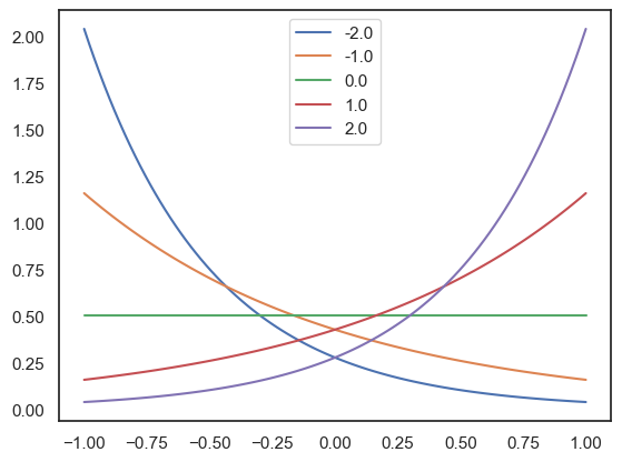

Appendix 2¶

Continuous Bernoulli distribution full derivation

Derivation of the exponential form of the continuous Bernoulli distribution, parametrized by the log odds L and adjusted to the [-1,1] interval.

$P(x; L) = \frac{e^{Lx}}{\int_{-1}^1 e^{Lx}} = \frac{e^{Lx}}{ \frac{e^L - e^{-L}}{L}} = L \frac{e^{Lx}}{2sinh(L)}$

Appendix 3¶

Visualization of the likelihood function with various parameters, in python.

delta = 100
s_i = np.linspace(-1, 1, delta)

fig, axes = plt.subplots(1, 3, figsize=(12, 3), sharey=True)
for idx, mu in enumerate([0.1, 0.5, 1]):
    for w_i in np.linspace(-2, 2, 5):
            p_mu = CB(s_i, w_i*mu)
            sns.lineplot(x=s_i, y=p_mu, ax=axes[idx], label=w_i).set(title=f"$\\mu={mu}$")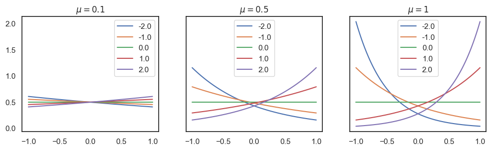

Appendix 4¶

Expected value of the $\mathcal{CB}$

\begin{align*} \mathbb{E}_{\mathcal{CB}(b)}[\sigma] &= \int \sigma \frac{ e^{b \sigma} }{ 2sinh(b) } d \sigma &= \frac{ b \left( \frac{(b-1)e^b}{b^2} + \frac{(b+1)e^-b}{b^2} \right) }{ 2sinh(b) } \\ &= \coth(b) - \frac{1}{b} \end{align*}

(1)

bs = np.linspace(-10, 10, 100)
plt.figure(figsize=(4, 1))
sns.lineplot(x=bs, y=1/np.tanh(bs) - 1/bs) # coth(b) - 1/b == 1/2 sech^2(b)
plt.show()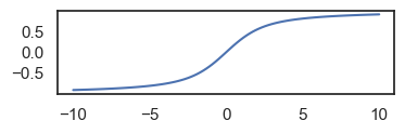

Appendix 5¶

Conservative dynamics

Let $x ∈ ℝ^n$ denote the system’s states (internal, blanket, and external states). The drift can be decomposed into a gradient part (from a potential U) and a solenoidal part R:

$ẋ = −∇U(x) + R(x)$

where $R = −Rᵀ$ is antisymmetric in state‐space.

The probability density $p(x, t)$ over states evolves according to the Fokker–Planck equation:

$∂ₜp(x,t) = −∇ · [ (−∇U + R) p(x,t) ] + diffusion terms.$

To determine the stationary distribution $p_s(x)$ , we set $∂ₜp(x,t) = 0$ . The Fokker-Planck equation then implies that the net probability current $J_s(x) = (−∇U(x) + R(x)) p_s(x) - D∇p_s(x)$ (assuming isotropic diffusion $D$ ) must be divergence-free: $∇ \cdot J_s(x) = 0$ . If we propose $p_s(x) = Z^{-1} \exp(−U(x)/D)$ (where $Z$ is a normalization constant), then the diffusive current $-D∇p_s(x)$ becomes $p_s(x)∇U(x)$ .

Substituting this into $J_s(x)$ , we get:

$J_s(x) = (−∇U(x) + R(x)) p_s(x) + p_s(x)∇U(x) = R(x) p_s(x)$ .

Thus, $p_s(x) \propto \exp(−U(x)/D)$ is the stationary distribution if and only if the solenoidal component of the probability current, $J_R(x) = R(x) p_s(x)$ , is itself divergence-free: $∇ \cdot (R(x) p_s(x)) = 0$ .

It is a key result from the study of non-equilibrium systems under the Free Energy Principle, particularly those possessing a Markov blanket and involving conservative particles, that this condition $∇ \cdot (R(x) p_s(x)) = 0$ holds (see Friston et al., 2023; but also related: Ao (2004); Xing (2010)). The conditional independence structure imposed by the Markov blanket, along with other FEP-specific assumptions (like conservative particles), constrains the system’s dynamics such that solenoidal forces $R(x)$ do not alter the Boltzmann form of the stationary distribution. Instead, they drive persistent, divergence-free probability currents $J_R(x)$ along iso-potential surfaces.

In steady state $(∂ₜp = 0)$ , only the gradient term $−∇U$ influences $p(x)$ . The stationary (nonequilibrium) distribution is

$p(x) ∝ exp{ −U(x) }$ ,

determined solely by the symmetric (potential) part −∇U. The antisymmetric $R$ does not reweight $p(x)$ ; it just circulates probability around isocontours of $U$ .

In most NESS systems, antisymmetric flows do alter the stationary measure. Under particular‐partition (Markov‐blanket) constraints, however, the internal–external factorization ensures that solenoidal (antisymmetric) flows remain divergence‐free, leaving the Boltzmann‐like steady distribution intact. This is why, in these Markov‐blanketed systems, one can have persistent solenoidal currents (nonequilibrium flows) yet preserve a stationary distribution that depends only on the symmetric part of the couplings.

Appendix 6¶

Detailed derivation of $\dfrac{\partial F}{\partial b_q}$

1. Subsitute our parametrization into F

Let’s start with substituting our parametrization into eq. .

1a. Accuracy term

From the RBM marginalization (eq. ):

$E(\bm{\sigma}) = \underbrace{-b_i\sigma_i - \sum_{j\neq i}J_{ij}\sigma_i\sigma_j}_{\text{Terms with } \sigma_i} \underbrace{-\sum_{j\neq i}b_j\sigma_j - \frac{1}{2}\sum_{j,k\neq i}J_{jk}\sigma_j\sigma_k}_{\text{Terms without } \sigma_i}$

Here, $-b_i\sigma_i$ becomes constant, since $\sigma_i$ is fixed. So we get:

$P(\sigma_{\backslash i}|\sigma_i) \propto \exp\left(\sum_{j\neq i}(b_j + J_{ij}\sigma_i)\sigma_j + \frac{1}{2}\sum_{j,k\neq i}J_{jk}\sigma_j\sigma_k\right)$

Taking expectation of $\ln P(\sigma_{\backslash i}|\sigma_i)$ under $q(σ_i)$ :

$\mathbb{E}q[\ln P(σ_{\backslash i}|σ_i)] = \text{const} + \sum_{j\neq i}b_jσ_j + S(b_q)\sum_{j\neq i}J_{ij}σ_j + \frac{1}{2}\sum_{j,k\neq i}J_{jk}σ_jσ_k$

Where $S(b_q) = \mathbb{E}_q[σ_i] = \coth b_q - 1/b_q$ is the expected value of the $\mathcal{CB}$ , a sigmoid function of the bias (#supplementary-information-4)).

1b. Complexity term

The complexity term in eq. is simply the KL-divergence term between two $\mathcal{CB}$ distributions. For $\mathcal{CB}$ distributions:

$q(x) = \frac{b_q}{2\sinh b_q}e^{b_q x},\quad p(x) = \frac{b}{2\sinh b}e^{b x}$

• KL divergence definition:

$D_{KL} = \int_{-1}^1 q(x) \ln\frac{q(x)}{p(x)} dx = \mathbb{E}_q[\ln q(x) - \ln p(x)]$

• Expand log terms:

$\ln q(x) = \ln b_q - \ln(2\sinh b_q) + b_q x$

$\ln p(x) = \ln b - \ln(2\sinh b) + b x$

• Subtract log terms:

$\ln\frac{q(x)}{p(x)} = \ln\frac{b_q}{b} + \ln\frac{\sinh b}{\sinh b_q} + (b_q - b)x$

• Take expectation under q(x):

$D_{KL} = \ln\frac{b_q}{b} + \ln\frac{\sinh b}{\sinh b_q} + (b_q - b)\mathbb{E}_q[x]$

• Compute expectation $\mathbb{E}_q[x]$ :

$\mathbb{E}_q[x] = \int_{-1}^1 x \frac{b_q e^{b_q x}}{2\sinh b_q} dx = \frac{1}{2\sinh b_q}\left[\frac{e^{b_q x}}{b_q^2}(b_q x - 1)\right]_{-1}^1$

• Evaluate at bounds:

$= \frac{1}{2\sinh b_q}\left(\frac{e^{b_q}(b_q - 1) - e^{-b_q}(-b_q - 1)}{b_q^2}\right)$

• Simplify using hyperbolic identities:

$= \frac{(b_q \cosh b_q - \sinh b_q)}{b_q^2 \sinh b_q} = \coth b_q - \frac{1}{b_q}$

• Final substitution for the complexity term:

$D_{KL} = \ln\frac{b_q \sinh b}{b \sinh b_q} + (b_q - b)\left(\coth b_q - \frac{1}{b_q}\right)$

1c. Combining the two terms

Combining the two terms, we get the following expression for the free energy:

$F = \ln\left(\frac{b_q}{b}\right) + \ln\left(\frac{\sinh(b)}{\sinh(b_q)}\right) + (b_q - b) S(b_q) - \sum_{j \ne i} \left( b_j + S(b_q) J_{ij} \right) \sigma_j - \dfrac{1}{2} \sum_{j \ne i} \sum_{k \ne i} J_{jk} \sigma_j \sigma_k + C$

where C denotes all constants in the equation that are independent of $\sigma or b_q$ .

2. Free Energy partial derivative calculation

• First, we differentiate the log terms:

$\frac{\partial}{\partial b_q}\left[\ln\frac{b_q}{b} + \ln\frac{\sinh b}{\sinh b_q}\right] = \frac{1}{b_q} - \coth b_q$

• Then, the KL core term:

$\frac{\partial}{\partial b_q}\left[(b_q - b)S(b_q)\right] = S(b_q) + (b_q - b)\frac{dS}{db_q}$

• The linear terms:

$\frac{\partial}{\partial b_q}\left[-\sum_{j≠i}(b_j + S(b_q)J_{ij})\sigma_j\right] = -\sum_{j≠i}J_{ij}\sigma_j\frac{dS}{db_q}$

• The constants vanish.

• Now, combining all terms:

$\frac{\partial F}{\partial b_q} = \left(\frac{1}{b_q} - \coth b_q\right) + \left(S(b_q) + (b_q - b)\frac{dS}{db_q}\right) - \sum_{j≠i}J_{ij}\sigma_j\frac{dS}{db_q}$

• Substituting $S(b_q) = \coth b_q - 1/b_q$ :

$= \left(\frac{1}{b_q} - \coth b_q\right) + \left(\coth b_q - \frac{1}{b_q} + (b_q - b)\frac{dS}{db_q}\right) - \sum_{j≠i}J_{ij}\sigma_j\frac{dS}{db_q}$

• Cancel terms:

$\cancel{\frac{1}{b_q}} \cancel{- \coth b_q} + \cancel{\coth b_q} \cancel{- \frac{1}{b_q}} + (b_q - b)\frac{dS}{db_q} - \sum_{j≠i}J_{ij}\sigma_j\frac{dS}{db_q}$

Gives us the final derivative:

$\frac{∂F}{∂b_q} = \left(b_q - b - \sum_{j\neq i}J_{ij}σ_j\right)\frac{dS}{db_q}$

Where $\frac{dS}{db_q} = -csch^2 b_q + \frac{1}{b_q^2}$ .

Setting the derivative to zero and solving for $b_q$ , we get: $b_q = b + \sum_{j \ne i} J_{ij} \sigma_j$

Now we remember that the expected value of the $\mathcal{CB}$ is the Langevin function of its bias -, $\mathbb{E}(x) = coth(b) - 1/b$ (). For simplicity, we will denote it as $L(x)$ . Now we can write:
$\mathbb{E}_{q}[\sigma_i] = L(b_q) = L \left( b + \sum_{j \ne i} J_{ij} \sigma_j \right)$

Q.E.D.

References¶

Friston, K., Da Costa, L., Sakthivadivel, D. A. R., Heins, C., Pavliotis, G. A., Ramstead, M., & Parr, T. (2023). Path integrals, particular kinds, and strange things. Physics of Life Reviews, 47, 35–62. 10.1016/j.plrev.2023.08.016
Ao, P. (2004). Potential in stochastic differential equations: novel construction. Journal of Physics A: Mathematical and General, 37(3), L25–L30. 10.1088/0305-4470/37/3/l01
Xing, J. (2010). Mapping between dissipative and Hamiltonian systems. Journal of Physics A: Mathematical and Theoretical, 43(37), 375003. 10.1088/1751-8113/43/37/375003