Simulation 1 - Self-orthogonalizing attractor neural networks emerging from the free energy principle

Simulation 1

A simple demonstration of the capabilities of FEP-based attractor networks¶

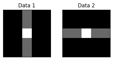
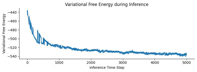
Here, we construct a network with 25 subparticles (representing 5x5 images) and train it with 2 different, but correlated images (Pearson’s r = 0.77, see Figure Figure 3B), with an precision of 0.1 and a learning rate of 0.01 (see next simulation for parameter-dependence). The training phase consisted of 500 epochs, each showing a randomly selected pattern from the training set through 10 time steps of simultaneous inference and learning. As shown on (fig. Figure 3B), local, micro-scale VFE minimization performed by the simultaneous inference and learning process leads to a macro-scale free energy minimization. Next, we obtained the attractor states corresponding to the input patterns by means of deterministic inference (updating with the expected value, instead of sampling from the $\mathcal{CB}$ distribution, akin to a vanilla Hopfield network). As predicted by theory, the attractor states were not simple replicas of the input patterns, but approximately orthogonalized versions of them, displaying a correlation coefficient of r=-0.19. Next, we demonstrated that the network (with stochastic inference) is not only able to retrieve the input patterns from noisy variations of them (fig. Figure 3C), but also generalizes well to reconstruct a third pattern, by combining its quasi-orthogonal attractor states (fig. Figure 3D). Note that this simulation only aimed to demonstrate some of the key features of the proposed architecture, and a comprehensive evaluation of the network’s performance, and its dependency on the parameters is presented in the next simulation.

Imports¶

import matplotlib.pyplot as plt
import numpy as np
import seaborn as sns

Construct training data¶

data1 = np.array([[0,0,1,0,0],
                  [0,0,1,0,0],
                  [0,0,4,0,0],
                  [0,0,1,0,0],
                  [0,0,1,0,0],
                 ])

data2 = np.array([[0,0,0,0,0],
                 [0,0,0,0,0],
                 [1,1,4,1,1],
                 [0,0,0,0,0],
                 [0,0,0,0,0],
                 ])

data1 = (data1 - data1.mean()) / data1.std()
data2 = (data2 - data2.mean()) / data2.std()

train_data = np.vstack(([data1.flatten(), data2.flatten()]))


# Convert lists to numpy arrays for plotting
arr1 = np.array(data1)
arr2 = np.array(data2)

# Create a figure with two subplots
fig, axes = plt.subplots(1, 2, figsize=(4, 2))

# Plot data1
im1 = axes[0].imshow(arr1, cmap='gray', vmin=0, vmax=2)
axes[0].set_title('Data 1')
axes[0].set_xticks([])
axes[0].set_yticks([])


# Plot data2
im2 = axes[1].imshow(arr2, cmap='gray', vmin=0, vmax=2)
axes[1].set_title('Data 2')
axes[1].set_xticks([])
axes[1].set_yticks([])


# Adjust layout and display the plot
plt.tight_layout()
plt.show()

Set up and train the network¶

We use a convenience functions to run and analyze the network, see simulation.utils.run_network for implementation details.

from simulation.utils import run_network, get_deterministic_attractors, continous_inference_and_learning

training_output = run_network(
            data=train_data,
            evidence_level=30,
            inverse_temperature=0.1,
            learning_rate=0.01,
            num_epochs=500,
            num_steps=10,
            progress_bar=False # Suppress progress bars within parallel runs
    )

Get attractors¶

attractors = get_deterministic_attractors(training_output[0], train_data, noise_levels=[0.0], inverse_temperature=1, plot=False)
import matplotlib.pyplot as plt
import numpy as np

num_attractors = len(attractors)
# Assuming attractors are 1D arrays that need reshaping.
# Infer shape from the first attractor, assuming it's a square image.
# Use the shape from the training data used to generate attractors
dim = int(np.sqrt(train_data.shape[1])) # e.g., sqrt(25) = 5

fig, axes = plt.subplots(1, num_attractors, figsize=(num_attractors * 2, 2.5)) # Adjusted figsize slightly

# Handle the case where there's only one attractor (axes might not be an array)
if num_attractors == 1:
    axes = [axes]

fig.suptitle("Determined Attractors") # Add a main title

for i, attractor in enumerate(attractors):
    # Reshape and plot
    # Use gray_r like in get_deterministic_attractors if needed, otherwise gray
    im = axes[i].imshow(attractor.reshape(dim, dim), cmap='gray')
    axes[i].set_title(f'Attractor {i+1}')
    axes[i].set_xticks([])
    axes[i].set_yticks([])
    # axes[i].set_axis_off() # Alternative to removing ticks

plt.tight_layout(rect=[0, 0.03, 1, 0.95]) # Adjust layout to prevent title overlap
plt.show()

# Also print the attractors array if needed for inspection
# attractors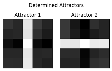

Compute attractor correlation coefficients¶

np.corrcoef(train_data)[0,1], np.corrcoef(attractors)[0,1]

(np.float64(0.7706422018348625), np.float64(-0.2043575361668949))

Visualize VFE¶

# Plot the Variational Free Energy (VFE) over time
vfe = training_output[5]
plt.figure(figsize=(8, 3))
plt.plot(vfe, label='VFE')
plt.xlabel("Inference Time Step")
plt.ylabel("Variational Free Energy")
plt.title("Variational Free Energy during Inference")
# plt.legend()
plt.tight_layout()
sns.despine()
plt.show()

Plot the network¶

nw = training_output[0]
nw.plot_network(node_size=5, edge_width=0.8)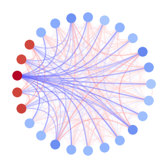

Test retrieval of noisy training data¶

nw = training_output[0]

test_pattern = np.array([[0,0,0,0,0],
                         [0,0,0,0,0],
                         [1,1,1,1,1],
                         [0,0,0,0,0],
                         [0,0,0,0,0],
                         ])
test_pattern = (test_pattern - test_pattern.mean()) / test_pattern.std()
test_pattern = test_pattern.flatten() * 1
test_pattern += np.random.normal(0, 0.5, test_pattern.shape)


acts, _, _, _, _ = continous_inference_and_learning(nw, data=test_pattern, 
                                                        inverse_temperature=1, 
                                                        learning_rate=0.0, 
                                                        num_steps=30)
    
attractors_np = np.array(attractors) # Shape (num_attractors, num_nodes)

acts_np = np.array(acts) # Shape (num_steps, num_nodes)

num_steps_inference = acts_np.shape[0]
num_attractors = attractors_np.shape[0]
num_nodes = attractors_np.shape[1]

# Calculate projections
projections = np.zeros((num_attractors, num_steps_inference))

for t in range(num_steps_inference):
    current_activation = acts_np[t]
    # Project current activation onto each attractor
    projections[:, t] = np.abs(np.dot(attractors_np, current_activation))
    # Optional: Normalize if needed, e.g., by norm of attractors
    # norms_sq = np.sum(attractors_np**2, axis=1)
    # projections[:, t] = np.dot(attractors_np, current_activation) / norms_sq


# Plotting the projections over time
plt.figure(figsize=(8, 3))
for k in range(num_attractors):
    # Assuming attractors correspond to the order in train_data (digits 0-9)
    plt.plot(projections[k, :], label=f'Attractor {k}') 

plt.xlabel("Inference Time Step")
plt.ylabel("Projection (Dot Product)")
plt.title("Projection of Network State onto Attractors during Inference")
#plt.legend(loc='center left', bbox_to_anchor=(1, 0.5)) # Place legend outside
# plt.grid(True, linestyle='--', alpha=0.6)
sns.despine()
plt.tight_layout()
plt.show()

Visualize the noisy training pattern¶

plt.figure(figsize=(4, 4))
plt.imshow(test_pattern.reshape(5, 5), cmap='gray', interpolation='nearest')
plt.title("New Prior")
plt.colorbar()
plt.show()

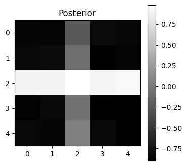
Visualize the posterior state¶

# Visualize the final state
final_state = np.mean(acts, axis=0)
plt.figure(figsize=(4, 4))
plt.imshow(final_state.reshape(5, 5), cmap='gray', interpolation='nearest')
plt.title("Posterior")
plt.colorbar()
plt.show()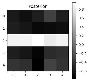

Generalize to new pattern¶



test_pattern = np.array([[0,0,1,0,0],
                         [0,0,1,0,0],
                         [1,1,1,1,1],
                         [0,0,1,0,0],
                         [0,0,1,0,0],
                         ])
test_pattern = (test_pattern - test_pattern.mean()) / test_pattern.std()
test_pattern = test_pattern.flatten() * 1


acts, _, _, _, _ = continous_inference_and_learning(nw, data=test_pattern, 
                                                        inverse_temperature=2, 
                                                        learning_rate=0.0, 
                                                        num_steps=20)
    
attractors_np = np.array(attractors) # Shape (num_attractors, num_nodes)

acts_np = np.array(acts) # Shape (num_steps, num_nodes)

num_steps_inference = acts_np.shape[0]
num_attractors = attractors_np.shape[0]
num_nodes = attractors_np.shape[1]

# Calculate projections
projections = np.zeros((num_attractors, num_steps_inference))

for t in range(num_steps_inference):
    current_activation = acts_np[t]
    # Project current activation onto each attractor
    projections[:, t] = np.abs(np.dot(attractors_np, current_activation))
    # Optional: Normalize if needed, e.g., by norm of attractors
    # norms_sq = np.sum(attractors_np**2, axis=1)
    # projections[:, t] = np.dot(attractors_np, current_activation) / norms_sq


# Plotting the projections over time
plt.figure(figsize=(8, 3))
for k in range(num_attractors):
    # Assuming attractors correspond to the order in train_data (digits 0-9)
    plt.plot(projections[k, :], label=f'Attractor {k}') 

plt.xlabel("Inference Time Step")
plt.ylabel("Projection (Dot Product)")
plt.title("Projection of Network State onto Attractors during Inference")
#plt.legend(loc='center left', bbox_to_anchor=(1, 0.5)) # Place legend outside
# plt.grid(True, linestyle='--', alpha=0.6)
sns.despine()
plt.tight_layout()
plt.show()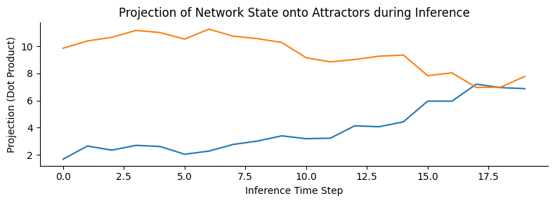

Visualize the test pattern¶

plt.figure(figsize=(4, 4))
plt.imshow(test_pattern.reshape(5, 5), cmap='gray', interpolation='nearest')
plt.title("New Prior")
plt.colorbar()
plt.show()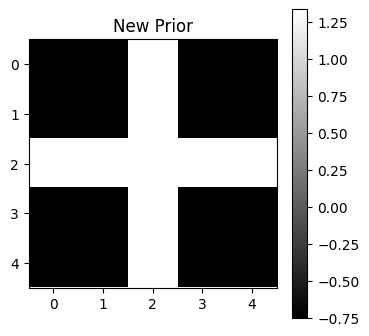

Visualize the posterior state¶

final_state = np.mean(acts, axis=0)
plt.figure(figsize=(4, 4))
plt.imshow(final_state.reshape(5, 5), cmap='gray', interpolation='nearest')
plt.title("Posterior")
plt.colorbar()
plt.show()